The name "transitive closure" means this:
We'll represent graphs using an adjacency matrix of Boolean values. We'll call the matrix for our graph G t(0), so that t(0)[i,j] = True if there is an edge from vertex i to vertex j OR if i=j, False otherwise. (This last bit is an important detail; even though, with standard definitions of graphs, there is never an edge from a vertex to itself, there is a path, of length 0, from a vertex to itself.)
Let n be the size of V. For k in 0..n, let t(k) be an adjacency matrix such that, if there is a path in G from any vertex i to any other vertex j going only through vertices in { 1, 2,..., k }, then t(k)[i,j] = True, False otherwise.
This set { 1, 2, ..., k } contains the intermediate vertices along the path from one vertex to another. This set is empty when k=0, so our previous definition of t(0) is still valid.
When k=n, this is the set of all vertices, so t(n)[i,j] is True if and only if there is a path from i to j through any vertex. Thus t(n) is the adjacency matrix for the transitive closure of G.
Now all we need is a way to get from t(0), the original graph, to t(n), the transitive closure. Consider the following rule for doing so in steps, for k >= 1:
t(k)[i,j] = t(k-1)[i,j] OR (t(k-1)[i,k] AND t(k-1)[k,j])In English, this says t(k) should show a path from i to j if
Transitive-Closure (G)
	n = |V|
	t(0) = the adjacency matrix for G

	// there is always an empty path from a vertex to itself,
	// make sure the adjacency matrix reflects this

	for i in 1..n do
		t(0)[i,i] = True
	end for

	// step through the t(k)'s

	for k in 1..n do
		for i in 1..n do
			for j in 1..n do
				t(k)[i,j] = t(k-1)[i,j] OR
					(t(k-1)[i,k] AND t(k-1)[k,j])
			end for
		end for
	end for
	return t(n)
This algorithm simply applies the rule n times, each time considering a new vertex through which possible paths may go. At the end, all paths have been discovered.
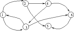
Let's look at an example of this algorithm. Consider the following graph:

So we have V = { 1, 2, 3, 4, 5, 6 } and E = { (1, 2), (1, 3), (2, 4), (2, 5), (3, 1), (3, 6), (4, 6), (4, 3), (6, 5) }. Here is the adjacency matrix and corresponding t(0):
down = "from"
across = "to"

adjacency matrix for G:               t(0):

  1 2 3 4 5 6                         1 2 3 4 5 6
1 0 1 1 0 0 0                       1 1 1 1 0 0 0
2 0 0 0 1 1 0                       2 0 1 0 1 1 0
3 1 0 0 0 0 1                       3 1 0 1 0 0 1
4 0 0 1 0 0 1                       4 0 0 1 1 0 1
5 0 0 0 0 0 0                       5 0 0 0 0 1 0
6 0 0 0 0 1 0                       6 0 0 0 0 1 1
Now let's look at what happens as we let k go from 1 to 6:
k = 1
add (3,2); go from 3 through 1 to 2
t(1) =
  1 2 3 4 5 6
1 1 1 1 0 0 0
2 0 1 0 1 1 0
3 1 1 1 0 0 1
4 0 0 1 1 0 1
5 0 0 0 0 1 0
6 0 0 0 0 1 1
k = 2
add (1,4); go from 1 through 2 to 4
add (1,5); go from 1 through 2 to 5
add (3,4); go from 3 through 2 to 4
add (3,5); go from 3 through 2 to 5
t(2) =
  1 2 3 4 5 6
1 1 1 1 1 1 0
2 0 1 0 1 1 0
3 1 1 1 1 1 1
4 0 0 1 1 0 1
5 0 0 0 0 1 0
6 0 0 0 0 1 1
k = 3
add (1,6); go from 1 through 3 to 6
add (4,1); go from 4 through 3 to 1
add (4,2); go from 4 through 3 to 2
add (4,5); go from 4 through 3 to 5
t(3) =
  1 2 3 4 5 6
1 1 1 1 1 1 1
2 0 1 0 1 1 0
3 1 1 1 1 1 1
4 1 1 1 1 1 1
5 0 0 0 0 1 0
6 0 0 0 0 1 1
k = 4
add (2,1); go from 2 through 4 to 1
add (2,3); go from 2 through 4 to 3
add (2,6); go from 2 through 4 to 6
t(4) =
  1 2 3 4 5 6
1 1 1 1 1 1 1
2 1 1 1 1 1 1
3 1 1 1 1 1 1
4 1 1 1 1 1 1
5 0 0 0 0 1 0
6 0 0 0 0 1 1
k = 5
t(5) =
  1 2 3 4 5 6
1 1 1 1 1 1 1
2 1 1 1 1 1 1
3 1 1 1 1 1 1
4 1 1 1 1 1 1
5 0 0 0 0 1 0
6 0 0 0 0 1 1
k = 6
t(6) =
  1 2 3 4 5 6
1 1 1 1 1 1 1
2 1 1 1 1 1 1
3 1 1 1 1 1 1
4 1 1 1 1 1 1
5 0 0 0 0 1 0
6 0 0 0 0 1 1
At the end, the transitive closure is a graph with a complete subgraph (a clique) involving vertices 1, 2, 3, and 4. You can get to 5 from everywhere, but you can get nowhere from 5. You can get to 6 from everwhere except for 5, and from 6 only to 5. Analysis This algorithm has three nested loops containing a
 (1) core,
so it takes
  (n3)
time.
What about storage? It might seem with all these matrices we
would need  (n3)
storage; however, note that at any point in the algorithm, we only need
the last two matrices computed, so we can re-use the storage from the
other matrices, bringing the storage complexity down to
 (n2).
(n2).
Another solution is called Floyd's algorithm (your book calls it "Floyd-Warshall"). We use an adjacency matrix, just like for the transitive closure, but the elements of the matrix are weights instead of Booleans. So if the weight of an edge (i, j) is equal to a, then the ijth element of this matrix is set to a. We also let the diagonal of the matrix be zero, i.e., the length of a path from a vertex to itself is 0.
A slight modification to Warshall's algorithm now solves this problem
in  (n3) time:
Floyd-Warshall (G)
	n = |V|
	t(0) = the weight matrix for edges of G,
			  with infinity if there is no edge

	// length of a path from vertex to itself is zero

	for i in 1..n do
		t(0)[i,i] = 0
	end for

	// step through the t(k)'s

	for k in 1..n do
		for i in 1..n do
			for j in 1..n do
				t(k)[i,j] = min (t(k-1)[i,j],
				     t(k-1)[i,k] + t(k-1)[k,j])
			end for
		end for
	end for
	return t(n)
Now, at each step, t(k)[i,j] is the length of the shortest path going through vertices 1..k. We make it either t(k-1)[i,j], or, if we find a shorter path via k, the sum of t(k-1)[i,k] and t(k-1)[k,j]. Of course, if there is no path from some i to some j, then for all k, we have t(k)[i,j] = infinity.
It's important to note that this  (n3)
asymptotic bound is tight, but that, for instance, running Dÿkstra's Algorithm
n times might be more efficient depending on the
characteristics of the graph. There is also another algorithm,
called Johnson's algorithm, that has asymptotically better performance
on sparse graphs. A tight lower bound for transitive closure
and all-pairs shortest-paths is
  (n2), because that's how many pairs there are and
we have to do something for each one.