The following algorithm can be used to implement problem reduction. It was described in Martelli and Montanari [1973], Martelli and Montanari [1978], and Nilsson [1980]. Nilsson calls it the AO* algorithm, the name we assume.

Rather than the two lists, OPEN and CLOSED, that were used in the A* algorithm, the AO* algorithm will use a single structure GRAPH, representing the part of the search graph that has been explicitly generated so far. Each node in the graph will point both down to its immediate successors and up to its immediate predecessors. Each node in the graph will also have associated with it an h' value, an estimate of the cost of a path from itself to a set of solution nodes. We will not store g (the cost of getting from the start node to the current node) as we did in the A* algorithm. It is not possible to compute a single such value since there may be many paths to the same state. And such a value is not necessary because of the top-down traversing of the best-known path, which guarantees that only nodes that are on the best path will ever be considered for expansion. So h' will serve as the estimate of goodness of a node.

1. Let GRAPH consist only of the node representing the initial state. (Call this node INIT.) Compute h'(INIT).
2. Until INIT is labeled SOLVED or until INIT's h' value becomes greater than FUTILITY, repeat the following procedure:

1. Trace the labeled arcs from INIT and select for expansion one of the as yet unexpanded nodes that occurs on this path. Call the selected node NODE.
2. Generate the successors of NODE. If there are none, then assign FUTILITY as the h' value of NODE. This is equivalent to saying that NODE is not solvable. If there are successors, then for each one (called SUCCESSOR), do the following:

1. Add SUCCESSOR to GRAPH.
2. If SUCCESSOR is a terminal node, label it SOLVED and assign it an h' value of 0.
3. If SUCCESSOR is not a terminal node, compute its h' value.

3. Propagate the newly discovered information up the graph by doing the following: Let S be a set of nodes that have been labeled SOLVED or whose h' values have been changed and so need to have values propagated back to their parents. Initialize S to NODE. Until S is empty, repeat the following procedure:

1. If possible, select from S a node none of whose descendants in GRAPH occurs in S. If there is no such node, select any node from S. Call this node CURRENT, and remove it from S.
2. Compute the cost of each of the arcs emerging from CURRENT. The cost of each arc is equal to the sum of the h' values of each of the nodes at the end of the arc plus whatever the cost of the arc itself is. Assign as CURRENT's new h' value the minimum of the costs just computed for the arcs emerging from it.
3. Mark the best path out of CURRENT by marking the arc that had the minimum cost as computed in the previous step.
4. Mark CURRENT SOLVED if all of the nodes connected to it through the new labeled arc have been labeled SOLVED.
5. If CURRENT has been labeled SOLVED or if the cost of CURRENT was just changed, then its new status must be propagated back up the graph. So add all of the ancestors of CURRENT to S.

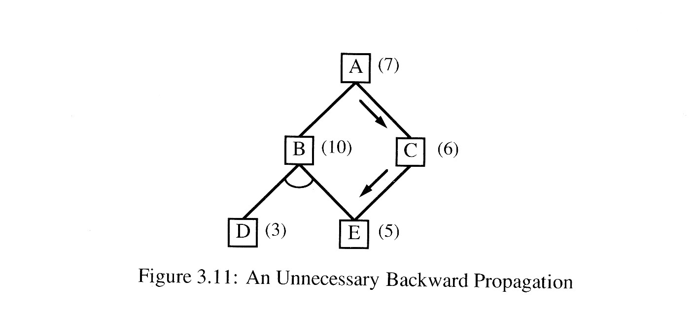It is worth noticing a couple of points about the operation of this algorithm. In step 2(c)v, the ancestors of a node whose cost was altered are added to the set of nodes whose costs must also be revised. As stated, the algorithm will insert all the node's ancestors into the set, which may result in the propagation of the cost change back up through a large number of paths that are already known not to be very good. For example, in Figure 3.11, it is clear that the path through C will always be better than the path through B, so work expended on the path through B is wasted. But if the cost of E is revised and that change is not propagated up through B as well as through C, B may appear to be better. For example, if, as a result of expanding node E, we update its cost to 10, then the cost of C will be updated to 11. If this is all that is done, then, when A is examined, the path through B will have a cost of only 11 compared to 12 for the path through C, and it will be labeled erroneously as the most promising path.

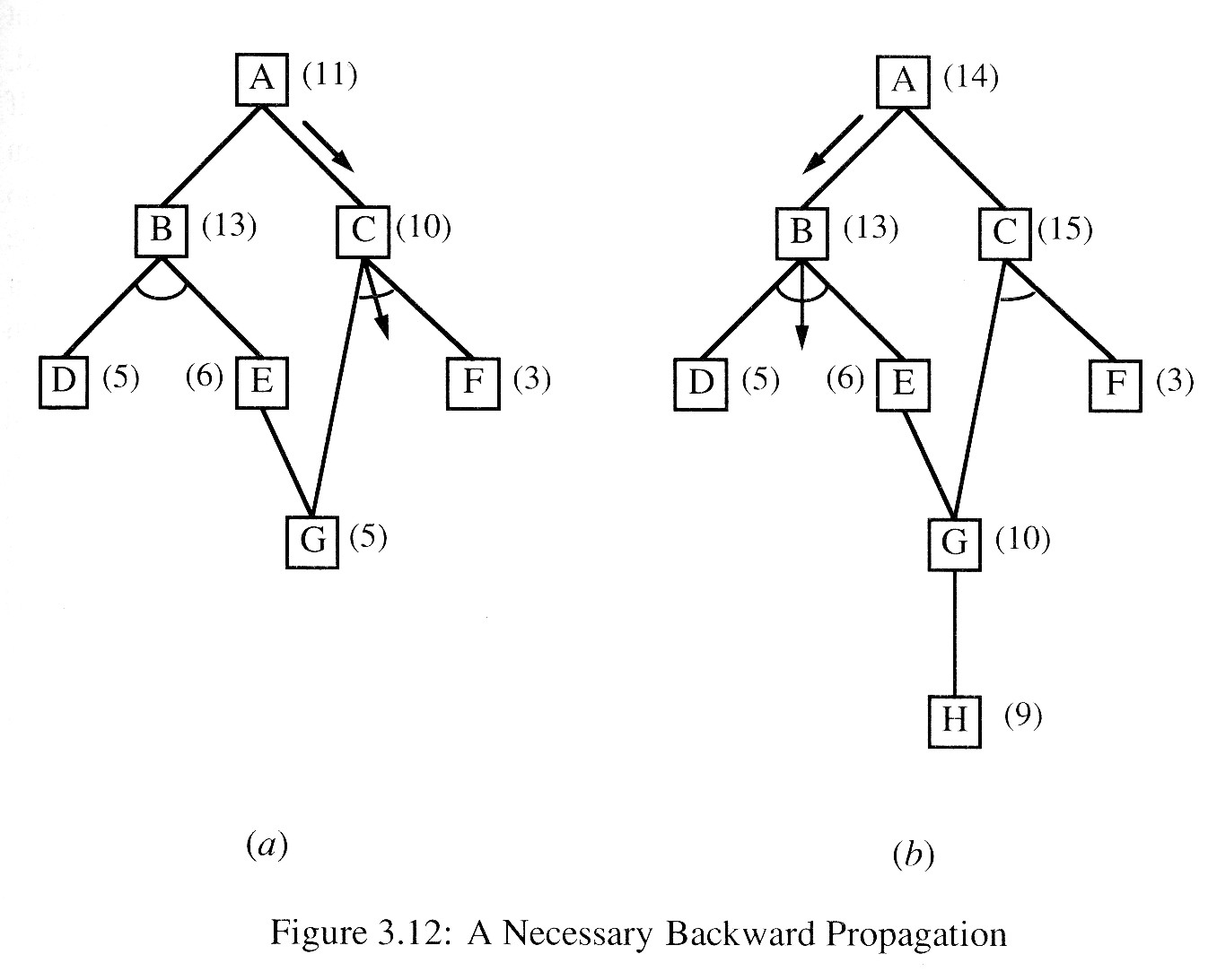In this example, the mistake might be detected at the next step, during which D will be expanded. If its cost changes and is propagated back to B, B's cost will be recomputed and the new cost of E will be used. Then the new cost of B will propagate back to A. At that point, the path through C will again be better. All that happened was that some time was wasted in expanding D. But if the node whose cost has changed is farther down in the search graph, the error may never be detected. An example of this is shown in Figure 3.12(a). If the cost of G is revised as shown in Figure 3.12(b) and if it is not immediately propagated back to E, then the change will never be recorded and a nonoptimal solution through B may be discovered.

A second point concerns the termination of the backward cost propagation of step 2(c). Because GRAPH may contain cycles, there is no guarantee that this process will terminate simply because it reaches the "top" of the graph. It turns out that the process can be guaranteed to terminate for a different reason, though. The proof of this is left as an exercise.