Assigned October 6.   Due October 25.

Description

Many rendering systems approximate the light arriving on the film plane by assuming a pin-hole camera, which produces images where everything that is visible is sharp.  In contrast, real cameras contain multi-lens assemblies with different imaging characteristics such as limited depth of field, field distortion, vignetting and spatially varying exposure.  In this assignment, you'll extend pbrt with support for a more realistic camera model that accurately simulates these effects.

Specifically, we will provide you with data about real wide-angle, normal and telephoto lenses, each composed of multiple lens elements. You will build a camera plugin for pbrt that simulates the traversal of light through these lens assemblies.  

With this camera simulator, you'll explore the effects of focus, aperture and exposure.  You will empirically characterize the critical points of the telephoto and normal lenses.  Using these data you can  optimize the performance of your simulator considerably.

Step 1

Read A Realistic Camera Model for Computer Graphics by Kolb, Mitchell, and Hanrahan.

Step 2: Compound Lens Simulator

• Copy this zip file to a directory at the same as the directory containing the 'core' directory.
  • A Makefile for Linux, and a Visual Studio 2003 project for Windows.
  • A stub C++ file, realistic.cpp, for the code you will write.
  • Six scene files, which end in .pbrt (the same as the .lrt files that have been used in previous assignments).
  • Four lens files, which end in .dat.
  • Binaries for a reference implementation of realistic.cpp on Linux, Windows and OSX.
  • Various textures used by the scene files.
• Modify the stub file, realistic.cpp, to trace rays from the film plane through the lens system supplied in the .dat files. The following is a suggested course of action, but feel free to proceed in the way that seems most logical to you:
  • Build an appropriate data structure to store the lens parameters supplied in the tab-delimited input .dat files. The format of the tables in these file is given in Figure 1 of the Kolb paper.
  • Develop code to trace rays through this stack of lenses. Please use a full lens simulation rather than the thick lens approximation in the paper. It's easier (you don't have to calculate the thick lens parameters) and sufficiently efficient for this assignment. Read and think about section 3 first, as it will probably be useful to be able to trace rays both forwards and backwards through the stack of lenses.
  • Write the RealisticCamera::GenerateRay function to trace randomly sampled rays through the lens system. For this part of the assignment, it will be easiest to just fire rays at the back element of the lens.  Some of these rays will hit the aperture stop and terminate before they exit the front of the lens.
  • Render images using commands such as 'pbrt dof-dragon.dgauss.pbrt'. Decrease the noise (and increase the rendering time) by changing the "integer pixelsamples" parameter in the scene files.
  • You may compare your output against the reference implementation, (realistic.so on Linux RedHat 9.0 and realistic.dll on Windows.

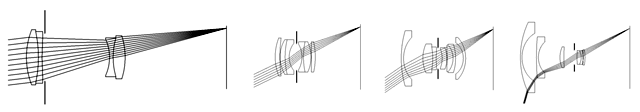
Sample Images:

• From left to right: telephoto, normal, wide angle and fisheye.
• Note that these were produced with 512 pixel samples rather than the default 32.
• Notice that the wide angle image is especially noisy -- why is that? Hint: look at the ray traces at the top of this web page.

Some conventions:

• Assume that the origin of the camera system is at the left-most element of the stack (the point closest to the world).
• Assume that the 'filmdistance' parameter passed to the RealisticCamera constructor is measured from the right-most element of the stack (the point closest to the film).
• There is exactly one aperture stop per lens data file.  This is the entry with a radius of 0. Note that the diameter of this entry is the maximum aperture of the lens. The actual aperture diameter to use is passed in the scene file, and appears as a parameter to the RealisticCamera constructor.
• In this assignment, everything is measured in millimeters.

Hints:

• ConcentricSampleDisk() is a useful function for converting two 1D uniform random samples into a uniform random sample on a disk. See p. 270 of the (old) PBRT book.
• It may be helpful to decompose the lens stack into individual lens interfaces and the aperture stop.  For the lens interfaces, you'll need to decide how to test whether rays intersect them, and how they refract according to the change of index of refraction on either side (review Snell's law).
• For rays that terminate at the aperture stop, return a ray with a weight of 0 -- pbrt tests for such a case and will terminate the ray.
• Be careful to weight the rays appropriately (this is represented by the value returned from GenerateRay). You should derive the weight from the integral equation governing irradiance incident on the film plane (hint: in the simplest form, this equation contains a cosine term raised to the fourth power). The exact weight will depend on the sampling scheme that you use to estimate this integral.  Make sure that your estimator is unbiased if you use importance sampling! The paper also contains details on this radiometric calculation.
• As is often the case in rendering, your code won't produce correct images until everything is working just right. Try to think of ways that you can modularize your work and test as much of it as possible incrementally as you go. Use assertions liberally to try to verify that your code is doing what you think it should at each step. Another wise course of action would be to produce a visualization of the rays refracting through your lens system as a debugging aid (compare to those at the top of this web page).

Step 3: Exploring the way a camera works with your simulator

In this section you'll explore how various choices affect focus, depth of field and exposure in your camera. Keep copies of your scenes that you use here, as you will email them to me.

1. The double gauss and telephoto lenses can be well approximated as a thick lens.
   1. Your first task is to determine the critical points of these lenses to characterize its thick lens approximation.  Compute these critical points by tracing rays that are parallel to the optical axis from the front and back of the lens stack, as described in the paper.; (These will give you the coordinates for D_P, D_P', D_F and D_F' in the diagram below, which you will report in your write-up). How do the parameters for the two lenses differ?
   2. Your second task is to verify your critical point calculation by taking an appropriate picture with the camera. The scene will consist of a depth of field target. The idea here is to take a picture of a ruler on a 45 degree angle. If the ruler intersects the plane of focus, then the sharpest point on the image of the ruler lets you deduce the depth of the conjugate plane. We have created a file, dof_target.pbrt, and a test scene, dof-test.pbrt, that includes this object. The scene is set up so that when you take a picture of the ruler the point of sharpest focus lets you read off the distance of the focal point from the front of the lens.  For example, the following image shows that the focal point is between 70 and 80 mm of the front of the ruler. The texture for the ruler is shown on the right.
      
      

      Your job is to modify dof-test.pbrt to produce a picture where the subject is projected at unit magnification onto the film plane (i.e. 1 mm on the subject appears as 1 mm on the film), and show that the focal depth is as expected given your critical point calculation. Specifically,

      1. Compute the values for D_X and D_X' in the following diagram that will produce an image at unit magnification.  Hint: at unit magnification, W = W'. (Why is that?)

         
         

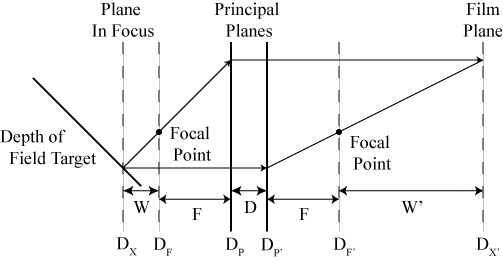
      2. Modify dof-test.pbrt so that the depth of field target at depth D_X will be visible in the output picture.  You will need to translate the target to get the appropriate focal depth in the frame. For example, if you calculate that D_X should be at 1000 mm away from the front of the lens (not shown), then you could translate the target away from the camera by 850 mm so that D_X would intersect the middle of the target (around the 15 cm mark). In addition, you will need to set the film depth so that the film plane intersects your computed D_X'.
      3. Render your scene and verify that the plane in focus in the rendered image and your chosen film plane indeed match your calculations for D_X and D_X'.

      Note: Taking a picture of a depth of field target in this way is a convenient way to characterize the critical points of a physical camera. In a real camera it isn't easy to trace parallel rays through the lens and measure where they cross the optical axis (as you did in step (a) above with your ray-tracer). Instead, the idea is that you move the depth of field target until the plane in focus is at roughly unit magnification. When this is achieved, the focal setting on the camera gives D_X', and the focal plane on the depth of field target gives D_X. Along with the observed magnification and focal length of the camera, F, you can calculate all the other variables in the diagram above, giving you the critical points.

2. Investigate depth of field. Use the telephoto lens for this test.
   1. Set up the camera so that it frames the depth of field target and is focused at 1 meter.  Now take two pictures, one with the aperture set at the maximum radius, and another with it stopped down to 1/2 its radius. How does the depth of field change?
   2. Now take two pictures with the aperture wide open.  One should be focused at 1 meter and the other at 2 meters.  How does the depth of field change?
3. Investigate exposure.  Render a scene (any scene you like) with the aperture full open and half open.  How does the exposure change? Does your ray tracer output the correct exposure?  Why or why not?

Step 4: Web page submission

1. In the archive that you downloaded in Step 1, you will find a "submission" directory. Copy this directory to your web space, and edit index.html to include your renderings and a description of your approach. The items that you have to replace are marked in green.
   • Please do NOT include your source code (you will email it to me, as described below).
   • Use exrtotiff to convert your .exr renderings to tiffs, and then convert these to jpgs to include in your web pages.
   • Though it is not a requirement, feel free to append a discussion of anything extra or novel that you did at the end of your web page.
2. Please send me an email containing
   • The URL of your web page
   • Your source code
   • Final scene files for Step 3.

FAQ

1. Q: PBRT complains that it can't find realistic.dll or realistic.so. What should I do?
   A: Make sure that '.' (the local directory) is in your PBRT_SEARCHPATH environment variable.  In this assignment, you will compile a camera plugin (realistic.so/dll) in your working directory. Note that the path is ':' delimited on Linux and ';' delimited on Windows.
2. Q: Should we be implementing the thick lens approximation described in the paper or a full lens simulation?
   A: Please implement the full lens simulation, which is less work for you and only slightly less efficient computationally.  Implementing the thick lens approximation is a superset of the work, since you need the full lens simulation in order to calculate the thick lens parameters.
3. Q: Why are my images so noisy?
   A: Integrating over the surface of the lens, especially for large apertures, requires multiple samples for accuracy.  Too few samples increases the variance of the integral estimate, resulting in noisy images.  The problem is exacerbated in Step 2 by the fact that you will fire many rays at the lens system that will not make it into the world because they will hit the aperture stop. To drive down the noise, you can increase the number of samples ("integer pixelsamples" parameter in the scene file).
4. Q: How can the value that you read off the depth of field target ruler be equal to the depth? It's on a 45 degree angle!
   A: Take a look at dof_target.pbrt. The ruler is scaled by sqrt(2), to allow you to read off the depth in this convenient way.

Miscellaneous Data

You can replace the cones in the rendered scenes with the dragons shown in Figures 6.6-6.9 in the (old) PBRT book. Copy the dragon.pbrt scene from the book CD, and comment out the appropriate lines in the hw3 directory scenes.  Be warned that this requires a fair amount of memory to render.

Grading

For each step (2 and 3)

** Passes all or almost all our tests.
* Substantial work was put in, but didn't pass all our tests.
0 Little or no work was done.

*** Extra credit may be given on a case-by-case basis for well done extensions (for any part of the project) that produce superior results.