Brian Kulis, Prateek Jain, Kristen Grauman
Summary
We introduce a method that enables
scalable similarity search for learned metrics. Given pairwise
similarity and dissimilarity constraints between some examples, we
learn a Mahalanobis distance function that captures the examples’
underlying relationships well. To allow sub-linear time similarity
search under the learned metric, we show how to encode the learned
metric parameterization into randomized locality-sensitive hash
functions. We further formulate an indirect solution that enables
metric learning and hashing for vector spaces whose high dimensionality
make it infeasible to learn an explicit transformation over the feature
dimensions. We demonstrate the approach applied to a variety of image
datasets, as well as a systems dataset. The learned metrics improve
accuracy relative to commonly-used metric baselines, while our hashing
construction enables efficient indexing with learned distances and very
large databases.
Overview of our approach
Motivation for searching with learned
metrics. A
good distance metric between images accurately reflects the true
underlying relationships, e.g., the category labels or other hidden
parameters. It should report small distances for examples that are
similar in the parameter space of interest (or that share a class
label), and large distances for unrelated examples. Recent advances in metric learning make it possible to
learn distance
functions that are more effective for a given problem, provided some
partially labeled data or constraints are available. Many
existing
metric learning algorithms learn the parameters of a Mahalanobis distance. By taking advantage
of the prior information, these techniques offer improved accuracy when
indexing examples.
Problem. How can we search efficiently with such a specialized learned metric? We want to be able to use these metrics to query a very large image database—potentially on the order of millions of examples or more. Certainly, a naive linear scan that compares the query against every database image is not feasible, even if the metric itself is efficient. Unfortunately, traditional methods for fast search (e.g, k-d trees, metric trees), cannot guarantee low query time performance for arbitrary specialized metrics.
Locality-Sensitive Hashing. We construct a new family of hash functions that will satisfy the locality-sensitivity requirement that is central to existing randomized algorithms [Indky & Motwani, STOC 1998, Charikar STOC 2002] for approximate nearest neighbor search. LSH guarantees sub-linear time retrieval with a bounded approximation error; the main idea is to derive a hash function such that the more similar two items are, the more likely they are to collide in the hash table. To use LSH for search, one must be able to provide a family of hash functions that are locality-sensitive for the similarity function of interest. See Figure 1.
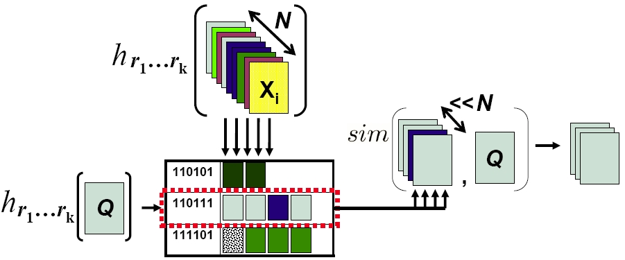 |
| Figure 1: Overview of locality-sensitive hashing (LSH [Indyk & Motwani 1999, Charikar 2002]). A list of k hash functions are applied to map N database examples into a hash table where similar items are likely to share a bucket. After hashing a query Q, one must only evaluate the similarity between Q and the database examples with which it collides to obtain the approximate nearest-neighbors. |
Our idea:
Semi-Supervised Locality-Sensitive Hash Functions. While existing hash functions could handle
similarity
measures such as Hamming distance, inner products, or L_p norms, our
main contribution is to derive hash functions that will respect the
learned Mahanobis distance or kernel function. We accomplish this
by
deriving hash functions that are "biased" according to the similarity
constraints
that train the metric: we want less similar examples to fall in
different hash buckets (even if the raw similarity between them
originally maps them to be close together), whereas we want more
similar examples to be more likely to fall into the same hash bucket
(even if the raw similarity suggested they were further apart).
See
Figure 2.
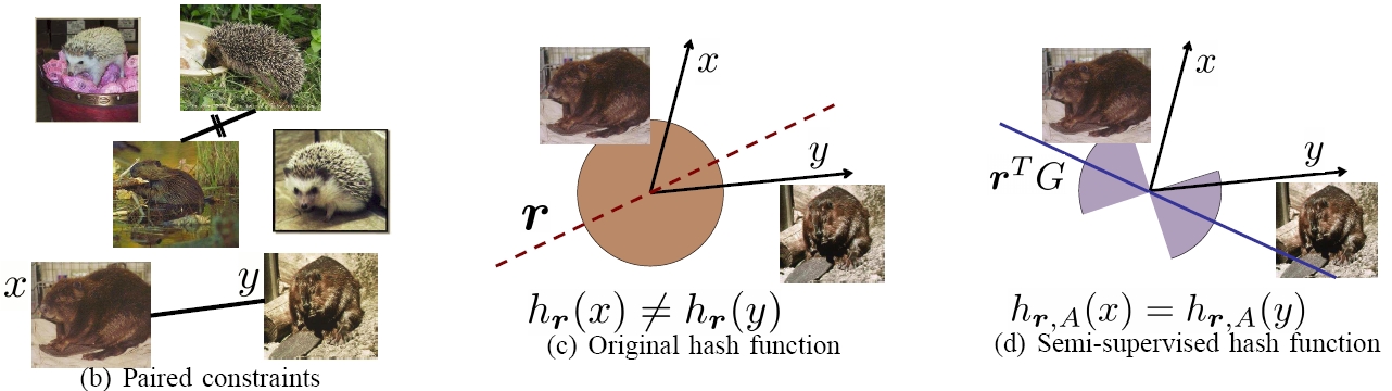 |
| Figure 2: (b) When learning a metric, some paired constraints can be obtained for a portion of the image database, specifying some examples that ought to be treated as similar (straight line) or dissimilar (crossed out line). (c) Whereas existing randomized LSH functions hash examples similar under the original distance together, (d) our semi-supervised hash functions incorporate the learned constraints, so that examples constrained to be similar—or other pairs like them—will with high probability hash together. The circular red region in (c) denotes that the existing LSH functions generate a hyperplane uniformly at random to separate images, in contrast, as indicated by the blue “hourglass” region in (d), our hash functions bias the selection of random hyperplane to reflect the specified (dis)similarity constraints. In this example, even though the measured angle between x and y is wide, our semi-supervised hash functions are unlikely to split them into different buckets since the constraints indicate they should be treated as similar. |
For
very high-dimensional data, explicit input space computations are
infeasible. We show how to compute the desired hash
function in terms of a series of weighted comparisons to the points
participating in similarity constraints---without needing to explicitly
access the learned Mahalanobis parameters.
Our method is applicable to general learned Mahalanobis metrics (e.g., where the initial "base metric" is Euclidean distance), and we also show how to embed two useful image matching kernels (PMK and PDK) so that they can be used with semi-supervised hash functions. See [Kulis et al. PAMI 2009 and Jain et al. CVPR 2008] for details.
While we are especially interested in the visual search problem, our algorithm is not specific to image features, and is also applicable to descriptors for other domains (e.g., text, bio, etc.).
Example results
The figures below show some example
results. Please see our papers for more examples.
 |
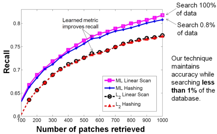 |
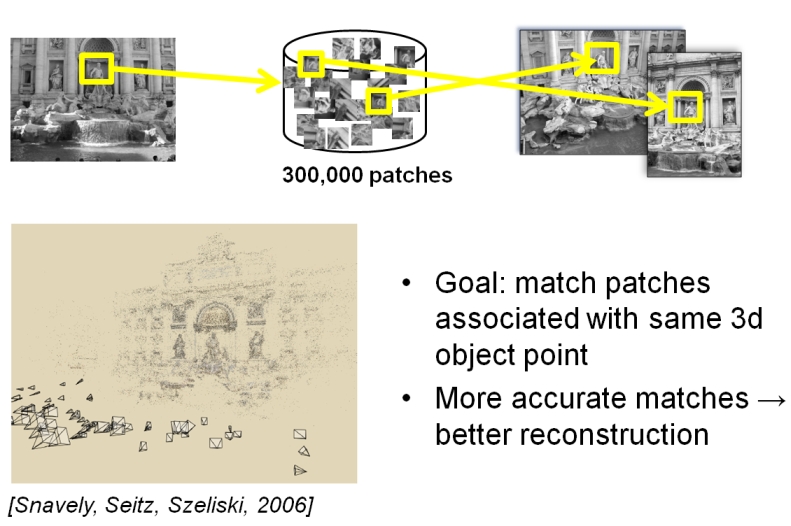
| Figure 3:
Result on the PhotoTourism patch dataset. We generate similarity
constraints based on true correspondences in the training data.
Given a new image, we want to search for similar patches. The
plot shows that the learned metric provides better retrieval of similar
patches, and that our semi-supervised hash functions make it possible
to search only a fraction of the entire pool to find the best matches. |
|
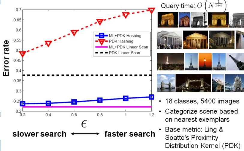 |
| Figure 4: Result on the Flickr Scenes dataset.
The goal is to take a query image and retrieve images of the same
tourist location. We generate similarity constraints based on
some labeled examples (same-class pairs form similarity constraints,
different-class pairs form dissimilarity constraints). The
learned proximity distribution kernel gives lower error (compare pink
curve to dotted black curve), and our semi-supervised hash functions
make it possible to search with that more accurate measure much more
efficiently (blue curve). For epsilon = 1.2, we are searching
only 3% of all the database images, and achieving an error rate very
close to linear scan's. |
Online extension
In [Jain
et
al.
NIPS 2008] we show how to dynamically update the hash tables as the
learned metric is updated in an online
manner. The above description assumes that the set of
similarity constraints have been given to us all at once.
However, in many real applications it may happen that new constraints
(supervision) are obtained gradually, and we want to be able to field
queries at any intermediate point in time. Rather than re-hash
all database examples from scratch once (which would take linear time
in the number of stored points), we introduce an algorithm to
incrementally update the hash keys for the stored data.
Essentially, we predict which bits in the keys are most likely to flip
given the adjustments to the constraints and learned distance
function. See Figure 4.
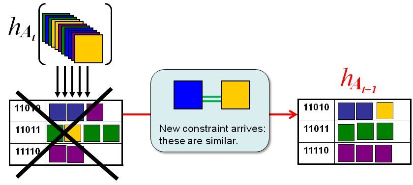 |
| Figure
4: If the hash table is constructed to
preserve the similarity according to a certain learned metric (A_t),
then once new similarity
constraints require updates to the metric
(A_{t+1}), the original hash table becomes obsolete. For
example, in this schematic, the points are originally arranged into the
buckets on the left. Then some new constraint comes in that says
"blue" and "yellow" points should be treated as similar. Note
that in the old hash table, blues and yellows did not share a
bucket.
Rather than simply rehash, we show how to dynamically update the hash
keys so that the revised metric is correctly preserved (with high
probability). |
References
Fast
Similarity Search for Learned Metrics. B. Kulis,
P.
Jain, and K. Grauman. In IEEE Transactions on Pattern
Analysis and Machine Intelligence (TPAMI), Vol. 31, No. 12, December,
2009. [link]
Fast Image Search for Learned Metrics. P. Jain, B. Kulis, and K. Grauman. In Proceedings of the IEEE Conference on Computer Vision and Pattern Recognition (CVPR), Anchorage, Alaska, June 2008. [pdf]
Online Metric Learning and Fast Similarity Search. P. Jain, B. Kulis,I. Dhillon, and K. Grauman.
In Advances in Neural Information Processing Systems
(NIPS), Vancouver, Canada, December 2008. [pdf]
Fast Image Search for Learned Metrics. P. Jain, B. Kulis, and K. Grauman. In Proceedings of the IEEE Conference on Computer Vision and Pattern Recognition (CVPR), Anchorage, Alaska, June 2008. [pdf]
Online Metric Learning and Fast Similarity Search. P. Jain, B. Kulis,
Acknowledgements: This work is supported in part by NSF CAREER IIS-0747356.