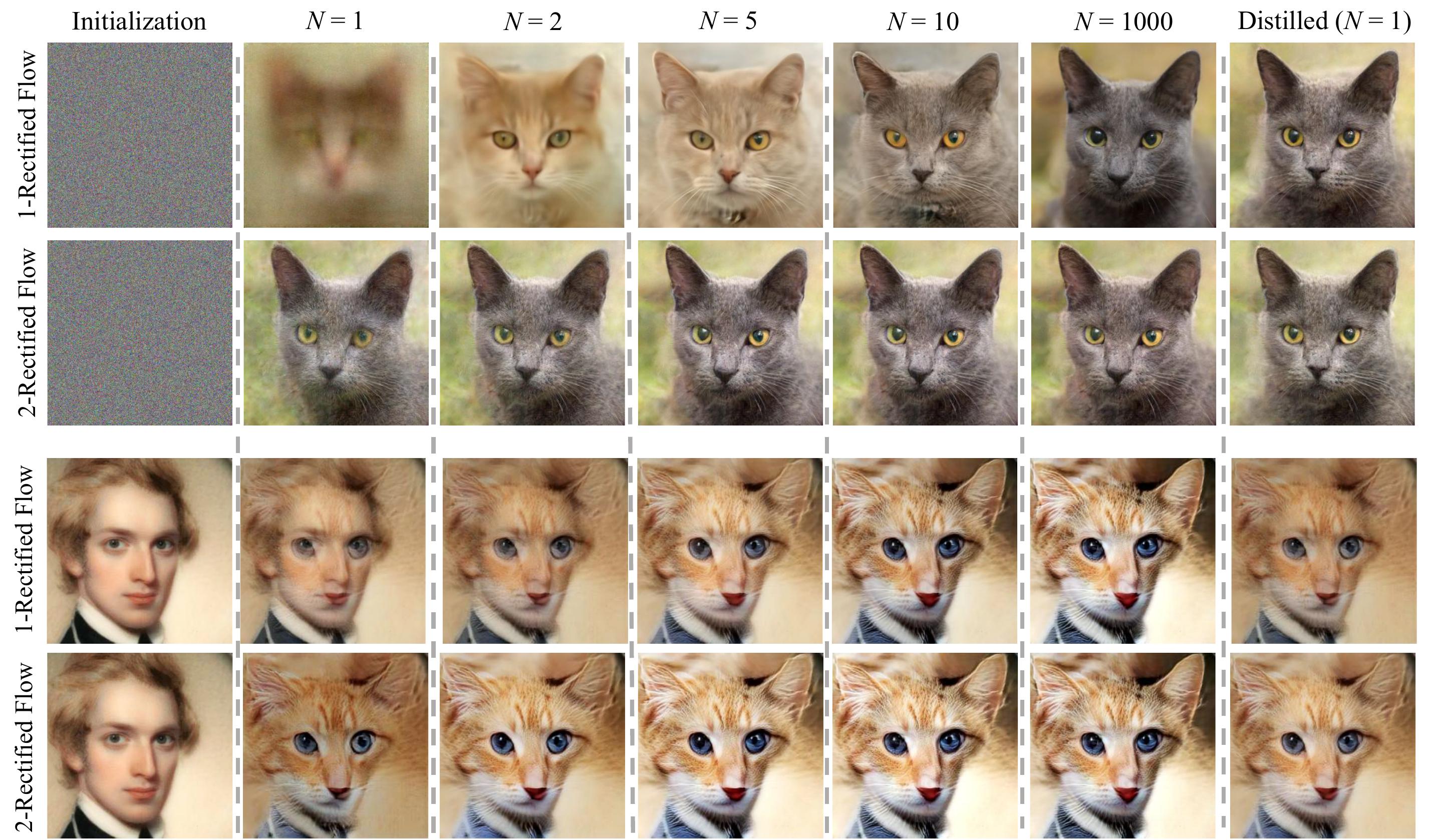Fig.1 - Rectified flow learns neural ODEs with straight trajectories for both generating (up two rows) and transferring (lower two rows) data, with a very small number $N$ of Euler steps (even a single step $N=1$).

Rectified Flow#

As distributions are the central object in statistics and machine learning, many fundamental learning problems, such as generative modeling and domain transfer, can be unifiedly viewed as finding a transport map to transfer one distribution to another. Rectified flow ([LGL22], [Liu22]) is a simple approach to finding a transport map between two empirically observed distributions by learning an ordinary differential equation (ODE), a.k.a. flow, model with the key idea of traveling in straight paths as much as possible.

This is closely related to the recent neural ODE and stochastic differential equation (SDE) models, especially the popular diffusion generative models and their ODE variants (e.g., [SSDK+20], [HJA20], and many more). The key idea here is to observe that there are infinitely many possible ODEs/SDEs to transfer the data between two given distributions, and each existing method implicitly picks their own trajectories without a clear criterion. Rectified flow, instead, places an explicit preference on the ODEs whose solution paths are straight lines (called straight flows). This yields a simple and principled framework with rich connections and implications to the optimal transport theory. Importantly, because straight flows incur no discretization error when solved numerically, the ODEs learned by rectified flow feature fast inference with a very small number of (or even a single) Euler steps. This allows us to achieve the inference speed similar to the traditional one-step generative models such as GAN/VAE, while benefiting from the nice properties of the ODE/SDE (or infinite-step) models during training.

Problem: Learning Transport Maps#

Here is the problem we are interested in:

The Transport Mapping Problem

Given empirical observations of two distributions $\pi_0, \pi_1$ on $\mathbb{R}^d$, find a transport map $T\colon\mathbb{R}^d\to\mathbb{R}^d$, which, in the infinite data limit, yields $Z_1 := T(Z_0)\sim \pi_1$ when $Z_0 \sim \pi_0$, that is, $(Z_0,Z_1)$ is a coupling (a.k.a transport plan) of $\pi_0$ and $\pi_1$.

Generative modeling: This is the case when $\pi_1$ is an empirically observed unknown distribution (of e.g., images), and $\pi_0$ an elementary distribution, such as the standard Gaussian distribution. We are interested in finding a nonlinear transform that turns a point drawn from $\pi_0$ to point that follows the data distribution $\pi_1$.
Transfer modeling: This is the case when both $\pi_0$ and $\pi_1$ are empirically observed unknown distributions, and we want to build a procedure to transfer a data point from $\pi_0$ to a point that follows $\pi_1$, or vice versa. This task admits enormous applications, such as domain adaption in transfer learning, image editing, and sim2real in robotics.

Given two distributions, there are often infinitely many transport maps $T$. Presumably, we hope to find a map that enjoys certain desirable practical properties, say high computational efficiency, besides doing the job of transferring $\pi_0$ to $\pi_1$. It is a critical problem to formulate the desirable properties mathematically and find efficient computational approaches to enforce them. One canonical approach is optimal transport (OT), which finds special couplings that are optimal in terms of minimizing a transport cost. In particular, Monge’s OT problem is

(1)#\[ \begin{align} \min_{T} \mathbb{E}[c(T(Z_0) - Z_0)] ~~~ s.t.~~~\mathrm{Law}(Z_0) = \pi_0,~ \mathrm{Law}(T(Z_0)) = \pi_1 \end{align} \]

where $c\colon\mathbb{R}^d\to\mathbb{R}$ is a cost function, e.g., $c(x) = \frac{1}{2}\lVert{x}\rVert^2$, and the $\mathbb{E}[c(T(Z_0) - Z_0)]$ measures the expected effort of transporting $Z_0$ to $Z_1=T(Z_0)$. Think $Z_0$ and $Z_1$ as two piles of sand and $c(Z_1-Z_0)$ the cost of transporting $Z_0$ to $Z_1$.

However, solving OT (1) is very challenging and it remains open to develop efficient algorithms for high dimensional and big data settings. Moreover, for generative and transfer modeling, the transport cost is in fact not of direct interest (as the learning performance is not directly related to the magnitude of $Z_1-Z_0$), even though the optimal transport maps induce nice smoothness properties that are beneficial for learning. Can we find alternative notions of optimality that are more directly related to ML tasks and easier to enforce in practice?

Method: Rectified flow#

Rectified flow learns the transport map $T$ implicitly by constructing an ordinary differential equation (ODE) driven by a drift force $v\colon \mathbb{R}^d \times [0,1]$:

(2)#\[ \begin{align} \mathrm{d}Z_t = v(Z_t, t) \mathrm{d}t,~~~~ t\in[0,1],~~~~ \text{starting from}~~~~ Z_0 \sim \pi_0, \end{align} \]

such that we have $Z_1 \sim \pi_1$ when following the ODE starting from $Z_0\sim \pi_0$. The main problem is how to construct the drift $v$ based on observations from $\pi_0$ and $\pi_1$, presumably using deep neural networks or other nonlinear approximators.

This appears to be a difficult problem. One natural approach is to find $v$ by minimizing $D(\rho_1^v;~ \pi_1)$, where $\rho_1^v$ is the distribution of $Z_1$ following the ODE with $v$, and $D(\cdot; ~\cdot)$ is a discrepancy measure, such as KL divergence. However, inferring (i.e., sampling or calculating the likelihood of) $\rho_1^v$ requires repeated simulation of the ODE, which is computationally expensive. The trouble here is that we do not know what intermediate trajectories the ODE should travel through before hand and hence need to infer it repeatedly.

Fortunately, this difficulty can be avoided by exploiting the over-parameterized nature of the problem: because we are only concerned with having the correct starting and terminal distributions $\pi_0$ and $\pi_1$, the intermediate distributions $\pi_t$ of $Z_t$ can be essentially an arbitrary smooth interpolation between $\pi_0$ and $\pi_1$. Hence, we can (and should) inject very strong priors on the intermediate trajectories, so that we can avoid the need for repeated inference, and also, as a bonus, incorporate proper beneficial propeties. Obviously, the simplest prior is straight trajectories. Straight paths are attractive both theoretically as an essential ingredient for achieving optimal transport, and computationally because ODEs with straight paths can be exactly simulated without time discretization.


Linear interpolation $X_t$	Rectified Flow $Z_t$	Straightened Rectified Flow

Fig.2 - Rectified flow between $\pi_0$ (magenta contour) and $\pi_1$ (red contour). Green and blue lines are the trajectories colored based on which mode of $\pi_0$ they are associated with for visualization.

Specifically, rectified flow works by finding an ODE to match (the marginal distributions of) the linear intepolation of points from $\pi_0$ and $\pi_1$. Assume we observe $X_0\sim \pi_0$ and $X_1 \sim \pi_1$. Let $X_t$ for $\forall t\in[0,1]$ be the linear (or geodesic) interpolation of $X_0$ and $X_1$:

\[ X_t = t X_1 + (1-t) X_0, ~~~~ t\in[0,1]. \]

Observe that $X_t$ follows a trivial ODE that already transfers $\pi_0$ to $\pi_1$:

(3)#\[ \begin{align} \mathrm{d}X_t = (X_1 - X_0) \mathrm{d}t, \end{align} \]

in which $X_t$ moves following the line direction $(X_1-X_0)$ with a constant speed. See Fig.2 (a).

However, this ODE does not solve the problem: it cann’t be simulated causally, because the update $X_t$ depends on the final state $X_1$, which is not supposed to be known at time $t<1$. In Fig. 2(a), the non-causality is reflected in the crossing points of the trajectories. When multiple trajectories intersect at a point $X_t$, the update direction is non-unique and hence can not modeled by the casual ODE in (2).

Hence, we want to "causalize" the interpolation process $X_t$, by “projecting” it to the space of causally simulatable ODEs of form $\mathrm{d} Z_t = v(Z_t, t) \mathrm{d} t $. A natural way to the L2 projection on the velocity field, finding $v$ by minimizing the least squares loss with the line directions $X_1-X_0$:

(4)#\[ \begin{align} \min_{v} \int_0^1 \mathbb{E}\left [\lVert{(X_1-X_0) - v(X_t, t)}\rVert^2\right] \mathrm{d}t. \end{align} \]

Theoretically, the solution can be represented using conditional expectation:

(5)#\[ \begin{aligned} v(z,t) = \mathbb{E}[X_1-X_0 ~|~X_t=z], \end{aligned} \]

which is the average of the directions of the lines passing through point $z$ at time $t$. We call the ODE with $v$ in (4) and (5) the rectified flow from induced from $(X_0,X_1)$.

In practice, we solve (4) with any off-the-shelf stochastic optimizer, such as SGD, by parameterizing $v$ with a neural network or other nonlinear models, and apporximating the expection $\mathbb{E}[\cdot]$ with empirical draws of $(X_0,X_1)$. See code here. For toy models, a simple kernel method works particularly well (code here).

As shown in Fig.2 (b), the trajectories $Z_t$ of rectified flow traces out the same density map as that of the interpolation trajectories $X_t$, but are rewired on the intersecting points to avoid the non-causality.

Key Properties

The ODE trajectories $Z_t$ and the interpolation $X_t$ have the same marginal distributions, that is,

\[\mathrm{Law}(Z_t) = \mathrm{Law}(X_t), ~~~ \forall t\in[0,1].\]

Hence, $(Z_0,Z_1)$ forms a coupling of $\pi_0$ and $\pi_1$.

$(Z_0,Z_1)$ guarantees to yield no larger transport cost than $(X_0,X_1)$ simultaneously for all convex cost functions $c$, that is,

\[\mathbb{E}[c(Z_1-Z_0)] \leq \mathbb{E}[c(X_1-X_0)],~~~ \text{$\forall$ convex $c\colon \mathbb{R}^d\to \mathbb{R}$}.\]

The data pair $(X_0,X_1)$ can be an arbitrary coupling of $\pi_0$ and $\pi_1$, typically independent (i.e., $(X_0,X_1)\sim \pi_0\times \pi_1$), obtained by randomly combining observations from $\pi_0$ and $\pi_1$. In comparison, the rectified coupling $(Z_0,Z_1)$ has a deterministic dependency as it is constructed from an ODE model. Hence, rectified flow converts an arbitrary coupling into a deterministic coupling with no larger convex transport costs.

Reflow: Fast Generation with Straight Flows#

Denote the rectified flow $\boldsymbol Z = \{Z_t: t\in[0,1]\} $ induced from $(X_0,X_1)$ by $\boldsymbol Z = \mathsf{Rectflow}((X_0,X_1))$. Applying this $\mathsf{Rectflow}(\cdot)$ operator recursively yields a sequence of rectified flows

\[ \boldsymbol Z^{k+1} = \mathsf{Rectflow}((Z_0^k, Z_1^k)) \]

with $(Z_0^0,Z_1^0)=(X_0,X_1)$, where $\boldsymbol Z^k$ is the $k$-th rectified flow, or simply $k$-rectified flow, induced from $(X_0,X_1)$. In practice, this can be implemented by drawing samples of $(Z_0^k, Z_1^k)$ from the $k$-th rectified flow, and using them to find the new flow by training procedure above (with $(X_0,X_1)$ replaced by $(Z_0^k,Z_1^k)$).

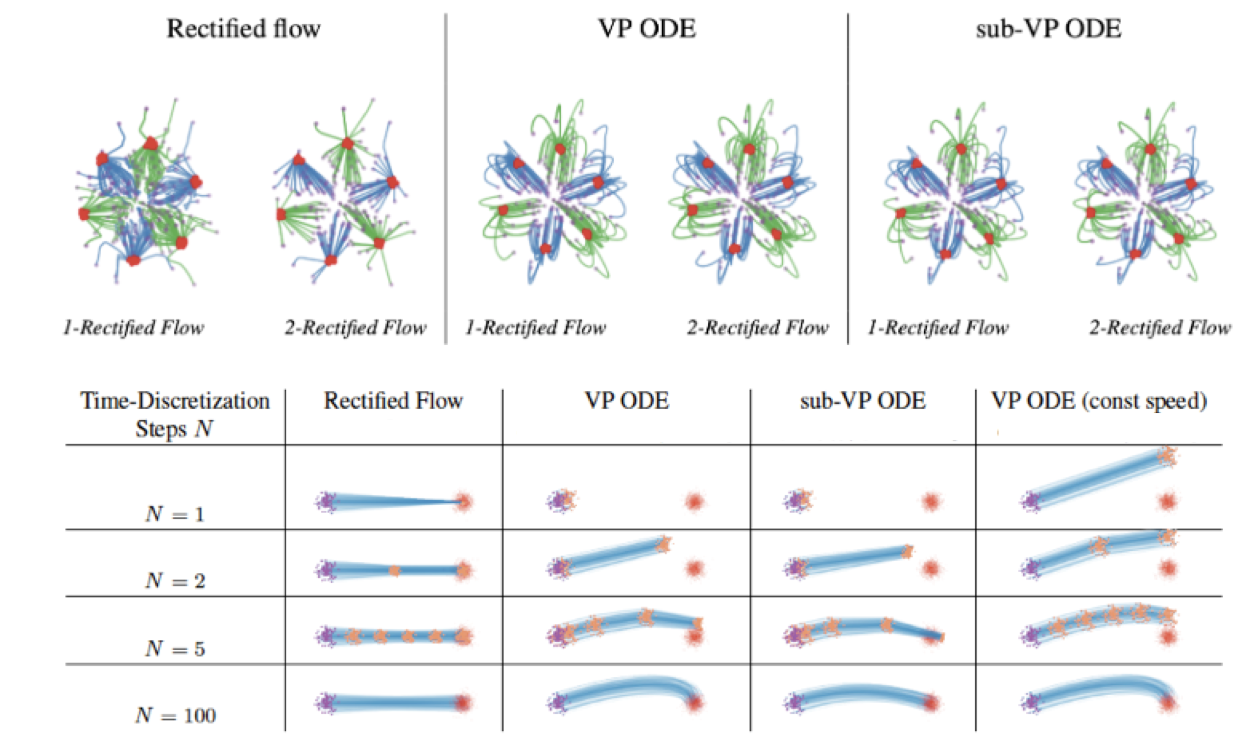
Besides decreasing transport cost shown above, this “reflow” procedure has the important effect of straightening paths of rectified flows: the paths of $\boldsymbol Z^k$ are increasingly straight as $k$ increases.

Key Properties (continued)

Measure the straightness of $\boldsymbol Z$ by $s(\boldsymbol{Z}) = \int_0^1 \mathbb{E}[\lVert Z_1-Z_0 - v(Z_t,t)\rVert^2]\mathrm{d}t$, such that $S(\boldsymbol Z) =0$ corresponds to straight paths. Then we have $\min_{k\leq K}S(\boldsymbol Z^k) = O(1/K)$.

Flows with nearly straight paths bring a key computational advantage as they incur small time-discretization error in numerical simulation. Indeed, if an ODE $\mathrm{d}Z_t = v(Z_t,t) \mathrm{d}t$ has perfectly straight paths, we have

\[ Z_t = Z_0 + t v(Z_0, 0), \]

meaning that the ODE can be solved exactly with a single Euler step, which addresses the very bottleneck of slow inference of ODE/SDE models. Hence, this reflow/straightnening procedure provides a special way for training one-step generative models (such as GAN/VAE), by leveraging ODEs as an intermediate step. For practical image generation, we find that it is sufficient to only reflow once.

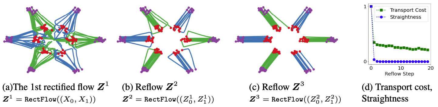
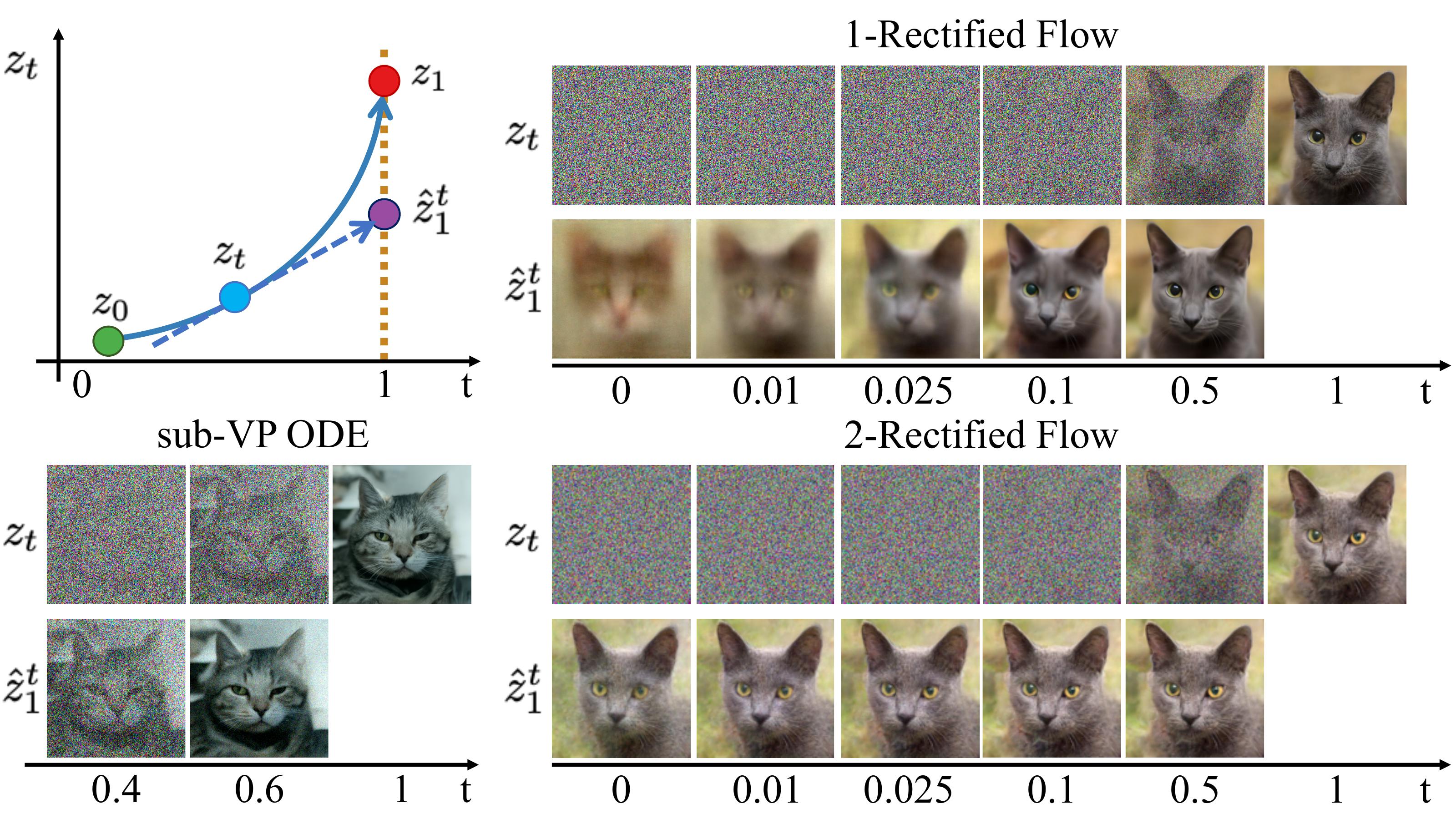Fig.3 - Sample trajectories $Z_t$ on the AFHQ Cat dataset. The extrapolation $\hat{Z}_1^t =Z_t + (1-t) v(Z_t, t)$ from different points $Z_t$ on the trajectories of 2-rectified flow are almost identical, indicating that its trajectory is almost straight.

Nonlinear Rectified Flows#

Rectified flow can be generalized to causalize any smooth interpolation process $X_t$ of $X_0$ and $X_1$. In this case, the velocity field should be constructed as

\[v(z,t) = \mathbb{E}[\dot X_t~|~X_t = z],\]

which is the expectation of the slope $\dot X_t$ for all the trajectories of $X_t$ that pass $z$ at time $t$. Obviously, $v$ can be estimated by solving

\[\min_v \int_0^1 \mathbb{E}\left [ \lVert{\dot X_t - v(X_t,t)}\rVert^2 \right ] \mathrm{d}t.\]

This generalization still yields the marginal preserving property, that is, $\mathrm{Law}(X_t) = \mathrm{Law}(Z_t)$ for $\forall t\in[0,1]$. But it no longer guarantees to decrease all convex transport costs, and it does not yield straight flows amenable to fast generation even with reflows.

It turns out that the probability flow ODEs [SSDK+20], including VP ODEs (equivalent to DDIM [HJA20]), sub-VP ODEs, and VE ODEs, can be viewed as special cases of this framework with $X_t = \alpha_t X_1 + \beta_t \xi$, with $\xi\sim \mathcal{N}(0,I)$ and proper choices of $\alpha_t$ and $\beta_t$ (see [LGL22] for details). As the slope $\dot X_t = \dot \alpha_t X_1+ \dot \beta_t \xi$ may depend on time $t$, these choices can yield curved trajectories and non-uniform update speed.

Diffusion Models#

$\newcommand{\d}{\mathrm{d}}$ In diffusion models, we learn a velocity field $v(z,t)$ to transfer $\pi_0$ to $\pi_1$ via a stochastic differential equation (SDE) of form

(6)#\[ \begin{align} \d Z_t = v(Z_t, t) \d t + \sigma(Z_t,t) \d W_t, \end{align} \]

where $\sigma(Z_t,t)$ is a diffusion coefficient and $W_t$ is a standard Brownian motion. Although ODEs $\d Z_t = v(Z_t,d) \d t $ is the special case of zero diffusion noise when $\sigma=0$, it is not much more limited in terms of representing marginal distributions: with the trick of converting between ODEs and SDEs in [SSDK+20], one can in principle convert the ODEs learned by rectified flow to an SDE with desirable a diffusion coefficient, without changing all marginal distributions. However, given that ODEs are coneptually simpler and faster to simulate, diffusion noise should be added only when it is clearly justified based on the problem of interest, based on Occam’s razor.

In a different, but ultmately equivalent view, the popular methods for training SDEs such as [SSDK+20] and [HJA20] can be viewed as special approaches that causalize non-smooth interpolation of $X_0$ and $X_0$ as shown in [Pel21] and [LWYL22].
The idea is to find a stochastic interpolation process $X_t$ of $X_0$ and $X_1$ that follows an (non-causal) SDE: $\d X_t = b(\boldsymbol X, t) \d t + \sigma(X_t, t)\d W_t.$ As the trajectory of a diffusion process, $X_t$ is an everywhere non-differentiable (or “rough’’) interoplation. With this, $v$ in (6) can be estimated as $v(z,t) = \mathbb{E}[b(\boldsymbol X,t)~|~ X_t = z]$, or equivalently

\[ \min_v \int_0^1\mathbb{E} \left[ \lVert b(\boldsymbol X,t) - v(X_t,t) \rVert^2 \right] \d t. \]

In this case, one can show that

\[ v(z,t) = \mathbb{E}[b(\boldsymbol X, t)~|~X_t = z] = \lim_{s\to t^+}\mathbb{E}\left[\frac{X_s-X_t}{s-t} \bigg | X_t = z\right ]. \]

As $X_t$ is non- differentiable, we can not exchange the order of $\lim_{s\to t^+}$ and $\mathbb{E}[\cdot]$. But if we are allowed to do so, then we have $v(z,t) = \mathbb{E}[\dot X_t~|~X_t =z]$, which is what we have in non-linear rectified flow.

Optimal Transport#

Rectified flow is “aggressive” in that it attempts to decrease the transport cost for all convex functions $c$, without preferring or specifying any particular $c$. However, if we are interested in solving the optimal transport problem with a particular cost, say the canonical quadratic cost $c(x) = \frac{1}{2} \lVert{x}\rVert^2$, then we need to modify the rectified flow procedure to target the specific $c$ that we are interested in, perhaps with the cost of increasing the other costs.

It turns out this can be done with a simple modification of the procedure. For the quadratic cost $c(x) = \frac{1}{2}\lVert{x}\rVert^2$, we simply need to constraint the drift $v$ to be a gradient field during the optimization. Specifically, we set the drift force to be $v(z,t) = \nabla_z f(z,t)$ with $f$ solving

\[\min_f \int_0^1\mathbb{E}\left [\lVert{X_1-X_0 - \nabla f(X_t, t)}\rVert^2\right] \mathrm{d}t.\]

For a general convex cost function $c$, we just need to set $v(z,t) = \nabla c^*(\nabla f(z,t))$, where $c^*$ is the convex conjugate of $c$, and $f$ solves

\[\min_f \int_0^1\mathbb{E}\left [c(X_1-X_0) + c^*(\nabla f_t(X_t))) - (X_1 - X_0)^\top \nabla f_t(X_t)\right] \mathrm{d}t.\]

This loss function can be viewed as a form of Bregman divergence [BDG04], or the so called matching loss used in learning generalized linear models [AHW95]. Denote by $\boldsymbol Z = $c$\text{-}\mathsf{Rectflow}((X_0,X_1))$, then recursively applying this mapping as the reflow procedure before guarantees to yield a $c$-optimal coupling in (1) at the fixed point. This is certainly closely related to Benamou-Breiner formulation and all the dynamic optimal transport stuffs. See more in [LGL22].

Epilogue#

Overall, rectified flow provides a pretty simple and clean framework for learning transport mappings from data.

It provides a simple and unified treatment for both generative and transfer modeling.
By learning straight flows, it provides a principled approach to learning ODEs with fast inference, effectively training one-step models with ODEs as intermediate steps.
The theoretical and algorithmic insights to optimal transport are of independent interest.
It provides a new way for understanding the popular diffusion models and their ODE variants.
It is purely ODE-based, avoiding the more mathematically sophistic SDE models both conceptually and algorithmically.
The idea of causalizing interpolation processes provides a principled framework for statistical learning and is amenable to rigorous theoretical analysis.

References#

LGL22(1,2,3): Xingchao Liu, Chengyue Gong, and Qiang Liu. Flow straight and fast: learning to generate and transfer data with rectified flow. arXiv preprint arXiv:2209.03003, 2022.
Liu22: Qiang Liu. Rectified flow: a marginal preserving approach to optimal transport. preprint, 2022.
SSDK+20(1,2,3,4): Yang Song, Jascha Sohl-Dickstein, Diederik P Kingma, Abhishek Kumar, Stefano Ermon, and Ben Poole. Score-based generative modeling through stochastic differential equations. In International Conference on Learning Representations. 2020.
HJA20(1,2,3): Jonathan Ho, Ajay Jain, and Pieter Abbeel. Denoising diffusion probabilistic models. Advances in Neural Information Processing Systems, 33:6840–6851, 2020.
Pel21: Stefano Peluchetti. Non-denoising forward-time diffusions. https://openreview.net/forum?id=oVfIKuhqfC, 2021.
LWYL22: Xingchao Liu, Lemeng Wu, Mao Ye, and Qiang Liu. Let us build bridges: understanding and extending diffusion generative models. arXiv preprint arXiv:2208.14699, 2022.
BDG04: Arindam Banerjee, Inderjit Dhillon, and Joydeep Ghosh. Clustering with bregman divergences. Journal of Machine Learning Research, 6:, 06 2004. doi:10.1137/1.9781611972740.22.
AHW95: Peter Auer, Mark Herbster, and Manfred K. Warmuth. Exponentially many local minima for single neurons. In NIPS. 1995.