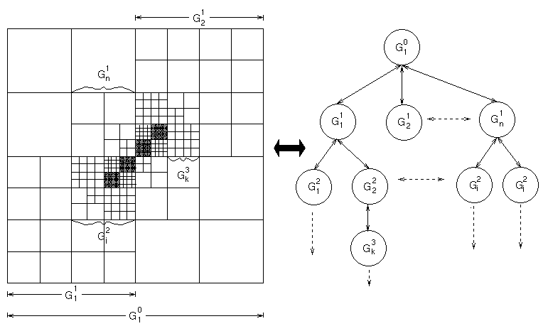
There are several algorithms that use the adaptive mesh refinement techniques. In our tutorial we give an example of one such algorithm - the Berger-Oliger Method [Berger, M.J. & Oliger, J. (1984) J.Comp.Phys., 53, 484-512] which is well suited for the solution of hyperbolic partial differential equations. In their original paper Berger and Oliger implemented their algorithm in one and two dimensions, but this method can be extended to higher dimensions in a straightforward way.
The algorithm starts with a rectangular coarse grid. As the solution progresses grid points with high local truncation errors are flagged. Fine grids are created such that all the flagged points are interior to some fine grid. The flagged points are clustered so that the area of the fine grids is minimized.
The fine grids are rectangles. In the original algorithm, these rectangles are rotated with respect to the orientation of the underlying coarse grid. In our implementation of the algorithm, we use rectangles (or cubes for the 3-dimensional cases) whose sides are parallel to the coordinate axes. The advantage of using rectangles (or cubes) is that one can use the same integrator for both the coarse and fine grid.
The fine grids have a separate identity from the underlying coarse grid. They have their own storage and solution vector. But the underlying coarse grid and the fine grid maintain a parent-child relation. Grid generation is applied at each grid level to the flagged points to build the next finer level of grids. For time dependent calculations as the regions that need refinement change so does the pattern of grids. Fine grid levels maybe deleted when not needed. Thus, new grids are created and old grids are destroyed in response to the computation.
If hl is the mesh spacing for a grid, then for a subgrid with just one higher level of refinement, the mesh spacing is hl+1 = hl / r. The refinement factor r is usually some multiple of 2. In practice the same refinement factor is used for all levels of refinement. A constant mesh ratio of the time step to space step is maintained on all the grids. This is achieved by using the same refinement factor for the time step as for the space step. The integration process is such that when one advances one grid step all its subgrids are integrated to the same time value.
The fundamental data structure that is used is a tree or a directed acylic graph of grids. Each grid in the grid hierarchy corresponds to a node in the tree. When a fine grid is nested within a coarse grid, the fine grid is called the child of the coarse grid. Subgrids of the same coarse grid and at the same level of refinement are called siblings. Subgrids at the same level of refinement but not having the same parents are called neighbors. There is a link between neighbors. This is shown in Figure 1.

The representations for two and three dimensional grid structures are more complex. Fine grids could be nested in more than one coarse grid. So a single parent node is replaced by a linked list of parent grids. Moreover, grids at the same level of refinement can overlap and hence a pointer to a list of intersecting grids is added to the information attached to each node.
The basic problem of grid generation can be stated as follows: given a list of flagged grid points how should rectangular subgrids be placed so that all the flagged points in a coarser grid are interior to some finer subgrid and the area of the subgrids is minimized? There could be several regions of a coarse grid that need refinement. A clustering algorithm groups these regions into a few clusters so that a single refined grid can be generated for all the regions in a cluster. The usual approach is to use a simple clustering algorithm that works in most cases. When the simple algorithm does not work a more expensive algorithm is tried.
A simple clustering algorithm is the nearest neighbor algorithm. This algorithm starts with one flagged point forming a cluster. Successive flagged points are added if the distance from those points to the cluster is less than a specified distance (say two mesh widths).
A more sophisticated algorithm connects the flagged points into a minimal spanning tree. The minimal spanning tree is a connected acyclic graph such that the sum of the edges is a minimum. A cluster is started with just one of the flagged points. The algorithm adds neighboring flagged points and fits a rotated rectangle immediately. The solution is evaluated, i.e. the ratio of the number of flagged grid points to the total number of coarse grid points covered by the fine grid is calculated. The solution gets a favorable evaluation if this ratio is high enough (typically between 1/2 and 3/4). The rectangle grows until there are no more flagged points or it receives an unfavorable evaluation. In case of an unfavorable evaluation a new rectangle is started.