The RF-LISSOM model is based on a simulated network of neurons with afferent connections from the external world and recurrent lateral connections between neurons. Connections adapt based on correlated activity between neurons. The result is a self-organized structure where afferent connection weights form a map of the input space, and lateral connections store long-term correlations in neuronal activity.
In RF-LISSOM, the cortical architecture has been simplified and reduced to the minimum necessary configuration to account for the observed phenomena. Because the focus is on the two-dimensional organization of the cortex, each ``neuron'' in the model cortex corresponds to a vertical column of cells through the six layers of the human cortex. This columnar organization helps make the problem of simulating such a large number of neurons tractable, and is viable because the cells in a column generally fire in response to the same inputs (chapter 2). Thus RF-LISSOM models biological mechanisms at an aggregate level, so it is important to keep in mind that RF-LISSOM ``neurons'' are not strictly identifiable with single cells in the human cortex.
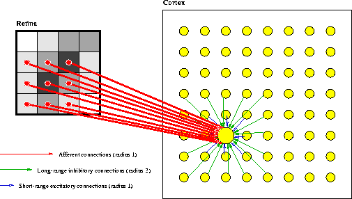
The cortical network is modeled with a sheet of interconnected neurons
and the retina with a sheet of retinal ganglion cells
(figure 3.1). Neurons receive afferent
connections from broad overlapping patches on the retina. The ![]() network is projected on to the retina of
network is projected on to the retina of ![]() ganglion cells, and each neuron is connected to ganglion cells in a
circular area of radius r around the projections. Thus, neurons at a
particular cortical location receive afferents from the corresponding
location on the retina. Depending on its location, the number of
afferents to a neuron varies from roughly
ganglion cells, and each neuron is connected to ganglion cells in a
circular area of radius r around the projections. Thus, neurons at a
particular cortical location receive afferents from the corresponding
location on the retina. Depending on its location, the number of
afferents to a neuron varies from roughly ![]() (at
the corners) to
(at
the corners) to ![]() (at the center).
(at the center).
In addition, each neuron has reciprocal excitatory and inhibitory lateral connections with itself and other neurons. Lateral excitatory connections are short-range, connecting each neuron and its close neighbors. Lateral inhibitory connections run for comparatively long distances, but also include connections from the neuron and its immediate neighbors to itself. Thus the ``lateral'' connections in the model are not exclusively from neurons located laterally, since they include self-recurrent connections.
The input to the model consists of 2-D patterns of activity representing retinal ganglion cell activations. Each ganglion cell is modeled only by its activation levels, not by its receptive field, so the input pattern is equivalent to an image after it has been processed by the retina. In addition, the transformation of retinal activation patterns by the LGN has been bypassed for simplicity, since LGN neurons do not change the shape of the receptive fields of the retina (chapter 2). Thus the ``retina'' of the model could equivalently be considered to represent a pattern of activity across neurons in the retinotopic map of the LGN.
The RF-LISSOM network will self-organize to represent the most common features present in the input images it has seen (Sirosh, 1995). Since tilt aftereffects appear to arise in the areas processing oriented inputs (chapter 2), simple oriented inputs (two-dimensional Gaussians) were used in the experiments presented in this thesis, as described in more detail in chapter 4.
The weights are initially set to random values or a smooth
distribution (such as a Gaussian profile), and are organized through
an unsupervised learning process. At each training step, neurons start
out with zero activity. The initial response ![]() of neuron
(i,j) is calculated as a weighted sum of the retinal activations:
of neuron
(i,j) is calculated as a weighted sum of the retinal activations:
where ![]() is the activation of retinal ganglion (a,b) within
the anatomical RF of the neuron,
is the activation of retinal ganglion (a,b) within
the anatomical RF of the neuron, ![]() is the corresponding
afferent weight, and
is the corresponding
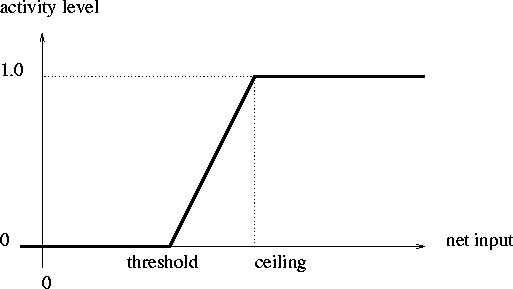
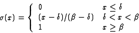
afferent weight, and ![]() is a piecewise linear approximation of
the sigmoid activation function (figure 3.2):
is a piecewise linear approximation of
the sigmoid activation function (figure 3.2):
Lateral interaction in the cortex sharpens neuronal response by
repeated exchange of activation
(Kohonen, 1989; Mountcastle, 1968). In RF-LISSOM, the
initial response evolves over a very short time scale through lateral
interaction. At each time step, the neuron combines the above
afferent activation ![]() with lateral excitation and
inhibition:
with lateral excitation and
inhibition:
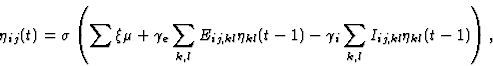
where Eij,kl is the excitatory lateral connection weight on the
connection from neuron (k,l) to neuron (i,j) , Iij,kl is the
inhibitory connection weight, and ![]() is the activity of
neuron (k,l) during the previous time step. All connection weights
are positive. The scaling factors
is the activity of
neuron (k,l) during the previous time step. All connection weights
are positive. The scaling factors ![]() and
and ![]() determine
the relative strengths of excitatory and inhibitory lateral
interactions. While the cortical response is settling, the retinal
activity remains constant.
determine
the relative strengths of excitatory and inhibitory lateral
interactions. While the cortical response is settling, the retinal
activity remains constant.
The activity pattern starts out diffuse and spread over a substantial part of the map, but within a few iterations of equation 3.3, converges into a small number of stable focused patches of activity, or activity bubbles. This sharpens the contrast between areas of high and low activity, helping it become focused around the maximally responding area.
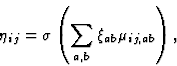
After the activity has settled, the connection weights of each neuron
are modified. Both afferent and lateral weights adapt according to the
same mechanism: the Hebb rule, normalized so that the sum of the
weights is constant:
![]()
where ![]() stands for the activity of neuron (i,j) in the
final activity bubble, wij,mn is the afferent or lateral
connection weight (
stands for the activity of neuron (i,j) in the
final activity bubble, wij,mn is the afferent or lateral
connection weight (![]() , E or I ),
, E or I ), ![]() is the learning rate
for each type of connection (
is the learning rate
for each type of connection (![]() for afferent weights,
for afferent weights,
![]() for excitatory, and
for excitatory, and ![]() for inhibitory) and Xmn
is the presynaptic activity (
for inhibitory) and Xmn
is the presynaptic activity (![]() for afferent,
for afferent, ![]() for lateral).
Afferent inputs, lateral excitatory inputs, and lateral inhibitory
inputs are normalized separately.
for lateral).
Afferent inputs, lateral excitatory inputs, and lateral inhibitory
inputs are normalized separately.
Following the Hebbian principle, the larger the product of the pre-
and post-synaptic activity ![]() , the larger the weight
change. Therefore, when the pre- and post-synaptic neurons fire
together frequently, the connection becomes stronger. Both excitatory
and inhibitory connections strengthen by correlated activity;
normalization then redistributes the changes so that the sum of each
weight type for each neuron remains constant. In effect, such a rule
distributes the weights of each neuron
, the larger the weight
change. Therefore, when the pre- and post-synaptic neurons fire
together frequently, the connection becomes stronger. Both excitatory
and inhibitory connections strengthen by correlated activity;
normalization then redistributes the changes so that the sum of each
weight type for each neuron remains constant. In effect, such a rule
distributes the weights of each neuron ![]() in the proportion
of its activity correlations with other neurons
in the proportion
of its activity correlations with other neurons ![]() ,
k,l=1..N .
,
k,l=1..N .
At long distances, very few neurons have correlated activity and therefore most long-range connections eventually become weak. The weak connections can be eliminated periodically by the researcher; through the weight normalization, this will concentrate the inhibition in a closer neighborhood of each neuron. The radius of the lateral excitatory interactions starts out large, but as self-organization progresses, it is decreased (according to a schedule set by the researcher) until it covers only the nearest neighbors. Such a decrease is necessary for global topographic order to develop and for the receptive fields to become well-tuned at the same time (for theoretical motivation for this process, see Kohonen 1982, 1989, 1993; Obermayer et al. 1992; Sirosh and Miikkulainen 1997; for neurobiological evidence, see Dalva and Katz 1994; Hata et al. 1993.) Together the pruning of lateral connections and decreasing excitation range produce activity bubbles that are gradually more focused and local. As a result, weights change in smaller neighborhoods, and receptive fields become better tuned to local areas of the retina.