Subsection 3.4.2 Systematic derivation of algorithms
¶We have described two algorithms for Gram-Schmidt orthogonalization: the Classical Gram-Schmidt (CGS) and the Modified Gram-Schmidt (MGS) algorithms. In this section we use this operation to introduce our FLAME methodology for systematically deriving algorithms hand-in-hand with their proof of correctness. Those who want to see the finer points of this methodologies may want to consider taking our Massive Open Online Course titled "LAFF-On: Programming for Correctness," offered on edX.
The idea is as follows: We first specify the input (the precondition) and ouput (the postcondition) for the algorithm. factorization
-
The precondition for the QR factorization is
\begin{equation*} A = \widehat A. \end{equation*}\(A \) contains the original matrix, which we specify by \(\widehat A \) since \(A \) will be overwritten as the algorithm proceeds.
-
The postcondition for the QR factorization is
\begin{equation} A = Q \wedge \widehat A = Q R \wedge Q^H Q = I . \label{chapter03-postcondition}\tag{3.4.1} \end{equation}This specifies that \(A \) is to be overwritten by an orthonormal matrix \(Q \) and that \(Q R \) equals the original matrix \(\widehat A \text{.}\) We will not explicitly specify that \(R \) is upper triangular, but keep that in mind as well.
Now, we know that we march through the matrices in a consistent way. At some point in the algorithm we will have divided them as follows:
where these partitionings are "conformal" (they have to fit in context). To come up with algorithms, we now ask the question "What are the contents of \(A \) and \(R \) at a typical stage of the loop?" To answer this, we instead first ask the question "In terms of the parts of the matrices are that naturally exposed by the loop, what is the final goal?" To answer that question, we take the partitioned matrices, and enter them in the postcondition (3.4.1):
(Notice that \(R_{BL} \) becomes a zero matrix since \(R\) is upper triangular.) Applying the rules of linear algebra (multiplying out the various expressions) yields
We call this the Partitioned Matrix Expression (PME). It is a recursive definition of the operation to be performed.
The different algorithms differ in what is in the matrices \(A \) and \(R \) as the loop iterates. Can we systematically come up with an expression for their contents at a typical point in the iteration? The observation is that when the loop has not finished, only part of the final result has been computed. So, we should be able to take the PME in (3.4.2) and remove terms to come up with partial results towards the final result. There are some dependencies (some parts of matrices must be computed before others). Taking this into account gives us two loop invariants:
-
Loop invariant 1:
\begin{equation} \begin{array}{l} \FlaOneByTwo{A_L}{A_R} = \FlaOneByTwo{Q_L}{\widehat A_R} \\ ~~~~~ \wedge \widehat A_L = Q_L R_{TL} \\ ~~~~~ \wedge Q_L^H Q_L = I \end{array}\label{chapter03-Inv1}\tag{3.4.3} \end{equation} -
Loop invariant 2:
\begin{equation*} \begin{array}{l} \FlaOneByTwo{A_L}{A_R} = \FlaOneByTwo{Q_L}{\widehat A_R - Q_L R_{TR} } \\ ~~~~~ \wedge \FlaOneByTwo{\widehat A_L}{\widehat A_R} = \FlaOneByTwo{Q_L R_{TL} }{Q_L R_{TR} + Q_R R_{BR}}\\ ~~~~~ \wedge Q_L^H Q_L = I \end{array} \end{equation*}We note that our knowledge of linear algebra allows us to manipulate this into
\begin{equation} \begin{array}{l} \FlaOneByTwo{A_L}{A_R} = \FlaOneByTwo{Q_L}{\widehat A_R - Q_L R_{TR} } \\ ~~~~~ \wedge \widehat A_L = Q_L R_{TL} \wedge Q_L^H \widehat A_L = R_{TR} \wedge Q_L^H Q_L = I . \end{array}\label{chapter03-Inv2}\tag{3.4.4} \end{equation}
The idea now is that we derive the loop that computes the QR factorization by systematically deriving the algorithm that maintains the state of the variables described by a chosen loop invariant. If you use (3.4.3), then you end up with CGS. If you use (3.4.4), then you end up with MGS.
Interested in details? We have a MOOC for that: LAFF-On Programming for Correctness.
