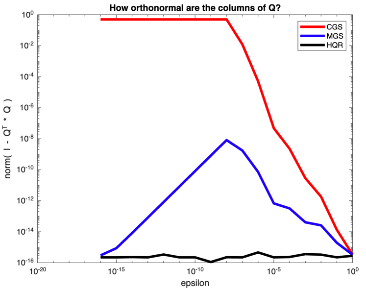
Subsection 3.3.7 Orthogonality of resulting \(Q \)
¶Homework 3.3.7.1.
Previous programming assignments have the following routines for computing the QR factorization of a given matrix \(A \text{:}\)
-
Classical Gram-Schmidt (CGS) Homework 3.2.3.1:
[ A_out, R_out ] = CGS_QR( A ).
-
Modified Gram-Schmidt (MGS) Homework 3.2.4.3:
[ A_out, R_out ] = MGS_QR( A ).
-
Householder QR factorization (HQR) Homework 3.3.4.3:
[ A_out, t_out ] = HQR( A ).
-
Form Q from Householder QR factorization Homework 3.3.5.2:
Q = FormQ( A, t ).
Use these to examine the orthogonality of the computed \(Q \) by writing the Matlab script Assignments/Week03/matlab/test_orthogonality.m for the matrix
Ponder This 3.3.7.2.
In the last homework, we examined the orthogonality of the computed matrix \(Q \) for a very specific kind of matrix. The problem with that matrix is that the columns are nearly linearly dependent (the smaller \(\epsilon \) is).
How can you quantify how close to being linearly dependent the columns of a matrix are?
How could you create a matrix of arbitrary size in such a way that you can control how close to being linearly dependent the columns are?
Homework 3.3.7.3. (Optional).
Program up your solution to Ponder This 3.3.7.2 and use it to compare how mutually orthonormal the columns of the computed matrices \(Q\) are.

