Subsection 4.3.3 Case 2: General case
¶ VIDEO Now we show how to use the SVD to find \(\hat x \) that satisfies
\begin{equation*}
\| b - A \hat x \|_2 = \min_x \| b - A x \|_2,
\end{equation*}
where \(\rank(A) = r \text{,}\) with no assumptions about the relative size of \(m \) and \(n \text{.}\) In our discussion, we let \(A = U_L \Sigma_{TL} V_L^H \) equal its Reduced SVD and
\begin{equation*}
A =
\left( \begin{array}{c | c}
U_L \amp U_R \end{array} \right)
\left( \begin{array}{c | c}
\Sigma_{TL} \amp 0 \\ \hline
0 \amp 0 \end{array} \right)
\left( \begin{array}{c | c}
V_L \amp V_R \end{array} \right)^H
\end{equation*}
its SVD.
The first observation is, once more, that an \(\hat x\) that minimizes \(\| b - A x \|_2 \) satisfies
\begin{equation*}
A \hat x = \hat b,
\end{equation*}
where \(\hat b = U_L U_L^H b \text{,}\) the orthogonal projection of \(b\) onto the column space of \(A \text{.}\) Notice our use of "an \(\hat x \)" since the solution won't be unique if \(r \lt m \) and hence the null space of \(A \) is not trivial. Substituting in the SVD this means that
\begin{equation*}
\left( \begin{array}{c | c}
U_L \amp U_R \end{array} \right)
\left( \begin{array}{c | c}
\Sigma_{TL} \amp 0 \\ \hline
0 \amp 0 \end{array} \right)
\left( \begin{array}{c | c}
V_L \amp V_R \end{array} \right)^H
\hat x = U_L U_L^H b.
\end{equation*}
Multiplying both sides by \(U_L^H \) yields
\begin{equation*}
\left( \begin{array}{c | c}
I \amp 0 \end{array} \right)
\left( \begin{array}{c | c}
\Sigma_{TL} \amp 0 \\ \hline
0 \amp 0 \end{array} \right)
\left( \begin{array}{c | c}
V_L \amp V_R \end{array} \right)^H
\hat x = U_L^H b
\end{equation*}
or, equivalently,
\begin{equation}
\Sigma_{TL} V_L^H \hat x = U_L^H b. \label{chapter04-LLS-general-1}\tag{4.3.1}
\end{equation}
Any solution to this can be written as the sum of a vector in the row space of \(A \) with a vector in the null space of \(A
\text{:}\)
\begin{equation*}
\hat x = V z =
\left( \begin{array}{c | c }
V_L \amp V_R
\end{array} \right)
\left( \begin{array}{c}{z_T}\\ \hline {z_B}
\end{array}\right)
=
\begin{array}[t]{c}
\underbrace{
V_L z_T}
\\
x_r
\end{array}
+
\begin{array}[t]{c}
\underbrace{
V_R z_B}
\\
x_n
\end{array}.
\end{equation*}
Substituting this into (4.3.1) we get
\begin{equation*}
\Sigma_{TL} V_L^H ( V_L z_T + V_R z_B ) = U_L^H b ,
\end{equation*}
which leaves us with
\begin{equation*}
\Sigma_{TL} z_T = U_L^H b .
\end{equation*}
Thus, the solution in the row space is given by
\begin{equation*}
x_r = V_L z_T = V_L \Sigma_{TL}^{-1} U_L^H b
\end{equation*}
and the general solution is given by
\begin{equation*}
\hat x = V_L \Sigma_{TL}^{-1} U_L^H b + V_R z_B,
\end{equation*}
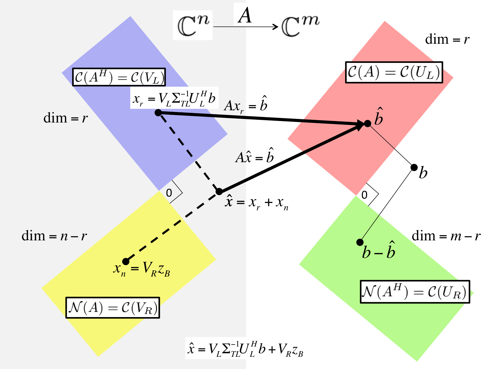
where \(z_B \) is any vector in \(\C^{n-r} \text{.}\) This reasoning is captured in Figure 4.3.3.1 .
PowerPoint Source Figure 4.3.3.1. Solving LLS via the SVD of \(A \text{.}\)
Homework 4.3.3.1 .
Reason that
\begin{equation*}
\hat x = V_L \Sigma_{TL}^{-1} U_L^H b
\end{equation*}
is the solution to the LLS problem with minimal length (2-norm). In other words, if \(x^\star \) satisfies
\begin{equation*}
\| b - A x^\star \|_2 = \min_x \| b - A x \|_2
\end{equation*}
then \(\| \hat x \|_2 \leq \| x^\star \|_2 \text{.}\)
Solution
The important insight is that
\begin{equation*}
x^\star =
\begin{array}[t]{c}
\underbrace{V_L \Sigma_{TL}^{-1} U_L^H b}\\
\hat x
\end{array}
+ V_R z_B
\end{equation*}
and that
\begin{equation*}
V_L \Sigma_{TL}^{-1} U_L^H b \quad \mbox{and} \quad
V_R z_B
\end{equation*}
are orthogonal to each other (since \(V_L^H V_R = 0\)). If \(u^H v = 0 \) then \(\| u + v \|_2^2 = \| u
\|_2^2 + \| v \|_2^2 \text{.}\) Hence
\begin{equation*}
\| x^\star \|_2^2 =
\| \hat x + V_R z_B \|_2^2 = \| \hat x \|_2^2
+ \| V_R z_B \|_2^2 \geq \| \hat x \|_2^2
\end{equation*}
and hence \(\| \hat x \|_2 \leq \| x^\star \|_2 \text{.}\)

