Subsection 3.1.1 Choosing the right basis
¶A classic problem in numerical analysis is the approximation of a function, \(f: \R \rightarrow \R \text{,}\) with a polynomial of degree \(n-1 \text{.}\) (The \(n-1 \) seems cumbersome. Think of it as a polynomial with \(n \) terms.)
* Now, often we know \(f \) only "sampled" at points \(\chi_0, \ldots, \chi_{m-1} \text{:}\)
In other words, input to the process are the points
and we want to determine the polynomal that approximately fits these points. This means that
This can be reformulated as the approximate linear system
which can be solved using the techniques for linear least-squares in Week 4. The matrix in the above equation is known as a Vandermonde matrix.
Homework 3.1.1.1.
Choose \(\chi_0, \chi_1, \cdots , \chi_{m-1} \) to be equally spaced in the interval \([ 0, 1 ] \text{:}\) for \(i = 0, \ldots, m-1 \text{,}\) \(\chi_i = i h\) ,where \(h = {1}/{(m-1)} \text{.}\) Write a Matlab code to create the matrix
as a function of \(n \) with \(m = 5000 \text{.}\) Plot the condition number of \(X \text{,}\) \(\kappa_2( X ) \text{,}\) as a function of \(n \) (Matlab's function for computing \(\kappa_2( X ) \) is cond( X ).)
You may want to use the recurrence \(x^{j+1} = x x^j\) and the fact that the .* operator in Matlab performs an element-wise multiplication.
Here is our implementation:
Assignments/Week03/answers/Vandermonde.m.(Assignments/Week03/answers/Vandermonde.m)
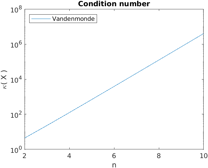
The graph of the condition number, \(\kappa( X ) \text{,}\) as a function of \(n\) is given by

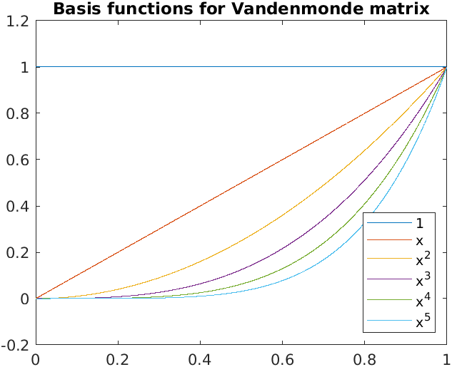
The parent functions \(1, x, x^2, \ldots \) on the interval \([ 0, 1 ] \) are visualized as
Notice that the curves for \(x^j \) and \(x^{j+1} \) quickly start to look very similar, which explains why the columns of the Vandermonde matrix quickly become approximately linearly dependent.
Think about how this extends to even more columns of \(A \text{.}\)
An alternative set of polynomials that can be used are known as Legendre polynomials. A shifted version (appropriate for the interval \([0,1] \)) can be inductively defined by
The polynomials have the property that
which is an orthogonality condition on the polynomials.
The function \(f: \R \rightarrow \R \) can now instead be approximated by
and hence given points
we can determine the polynomial from
This can be reformulated as the approximate linear system
which can also be solved using the techniques for linear least-squares in Week 4. Notice that now the columns of the matrix are (approximately) orthogonal: Notice that if we "sample" \(x \) as \(\chi_0, \ldots , \chi_{n-1} \text{,}\) then
which equals the dot product of the columns indexed with \(s\) and \(t \text{.}\)
Homework 3.1.1.2.
Choose \(\chi_0, \chi_1, \cdots , \chi_{m-1} \) to be equally spaced in the interval \([ 0, 1 ] \text{:}\) for \(i = 0, \ldots, m-1 \text{,}\) \(\chi_i = i h \text{,}\) where \(h = {1}/{(m-1)} \text{.}\) Write a Matlab code to create the matrix
as a function of \(n \) with \(m =5000 \text{.}\) Plot \(\kappa_2( X ) \) as a function of \(n \text{.}\) To check whether the columns of \(X \) are mutually orthogonal, report \(\| X^T X - D \|_2 \) where \(D\) equals the diagonal of \(X^T X \text{.}\)
Here is our implementation:
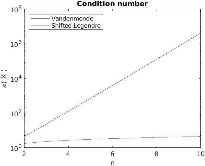
Assignments/Week03/answers/ShiftedLegendre.m. (Assignments/Week03/answers/ShiftedLegendre.m)The graph of the condition number, as a function of \(n\) is given by
We notice that the matrices created from shifted Legendre polynomials have a very good condition numbers.
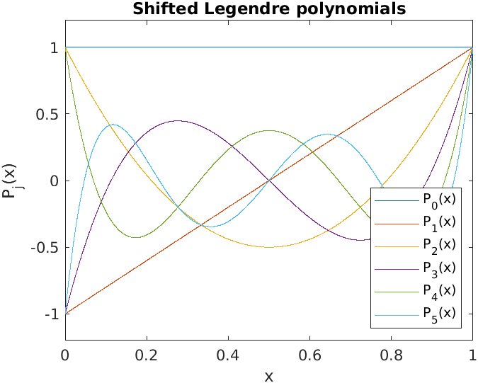
The shifted Legendre polynomials are visualized as

The columns of the matrix \(X \) are now reasonably orthogonal:
X^T * X for n=5:

ans =

        5000           0           1           0           1
           0        1667           0           1           0
           1           0        1001           0           1
           0           1           0         715           0
           1           0           1           0         556
Remark 3.1.1.1.
The point is that one ideally formulates a problem in a way that already captures orthogonality, so that when the problem is discretized ("sampled"), the matrices that arise will likely inherit that orthogonality, which we will see again and again is a good thing. In this chapter, we discuss how orthogonality can be exposed if it is not already part of the underlying formulation of the problem.
