Unit 1.4.2 Matrix-matrix multiplication via rank-1 updates
¶Homework 1.4.2.1.
Fill in the blanks:
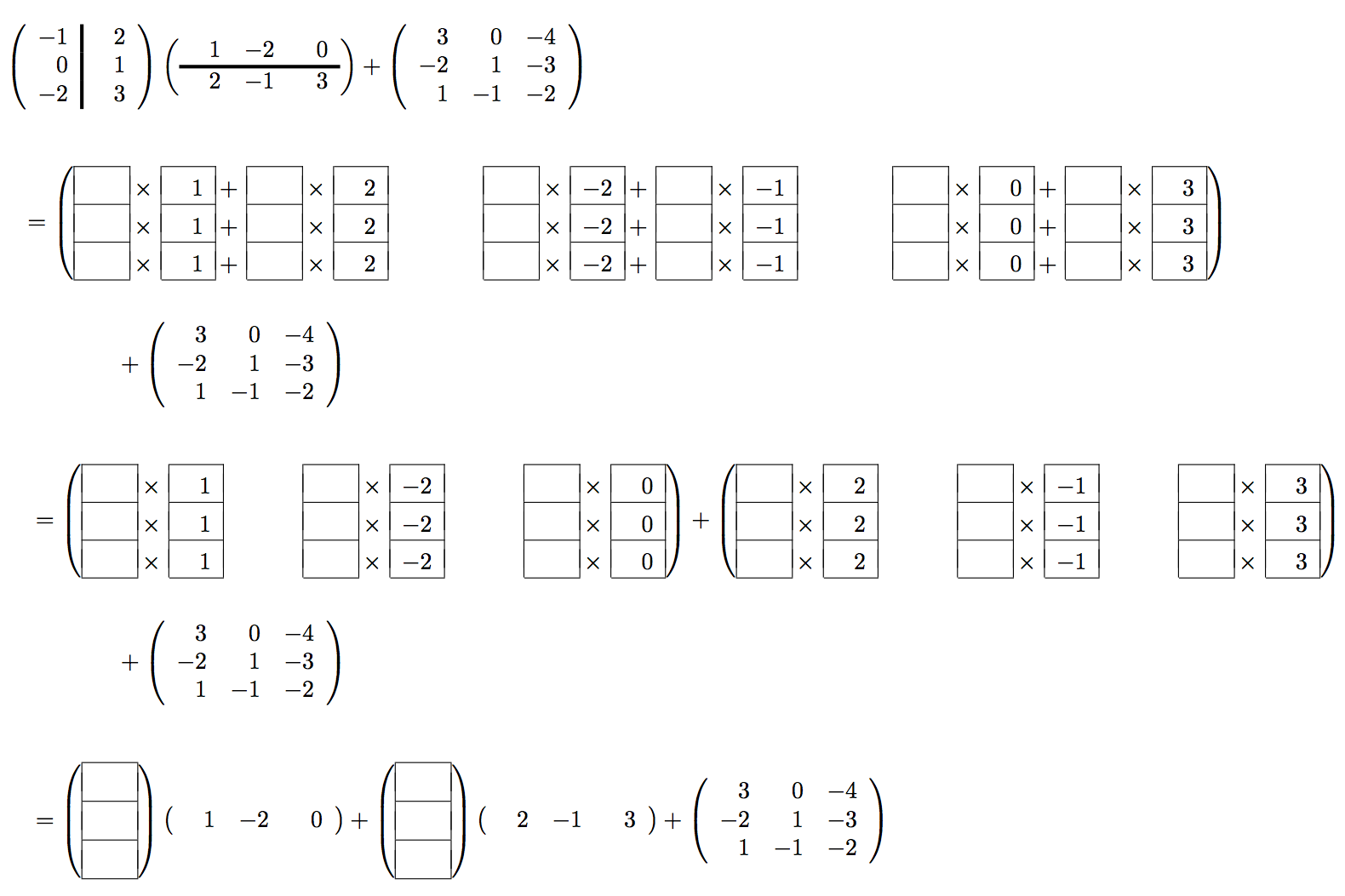
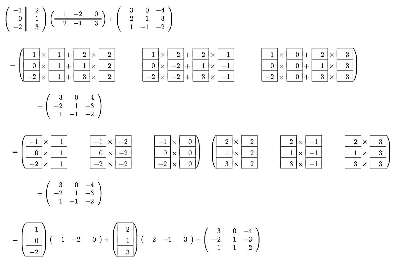
Let us partition \(A \) by columns and \(B \) by rows, so that
\begin{equation*}
\begin{array}{rcl}
C \amp:=\amp
\left( \begin{array}{c | c | c | c }
a_0 \amp a_1 \amp \cdots \amp a_{k-1}
\end{array} \right)
\left( \begin{array}{c}
\widetilde b_0^T \\ \hline
\widetilde b_1^T \\ \hline
\vdots \\ \hline
\widetilde b_{k-1}^T
\end{array} \right)
+
C
\\
\amp = \amp
a_0 \widetilde b_0^T
+
a_1 \widetilde b_1^T
+\cdots +
a_{k-1} \widetilde b_{k-1}^T
+ C
\end{array}
\end{equation*}
A picture that captures this is given by
\begin{equation*}
\begin{array}{l}
{\bf for~} p := 0, \ldots , k-1 \\[0.15in]
~~~
\left. \begin{array}{l}
{\bf for~} j := 0, \ldots , n-1 \\[0.15in]
~~~ ~~~
\left. \begin{array}{l}
{\bf for~} i := 0, \ldots , m-1 \\
~~~ ~~~ \gamma_{i,j} := \alpha_{i,p} \beta_{p,j} + \gamma_{i,j} \\
{\bf end}
\end{array} \right\} ~~~ \begin{array}[t]{c}
\underbrace{c_j := \beta_{p,j} a_p + c_j}\\
\mbox{axpy}
\end{array}
\\[0.2in]
~~~ {\bf end}
\end{array} \right\} ~~~ \begin{array}[t]{c}
\underbrace{C := a_p \widetilde b_p^T + C}\\
\mbox{rank-1 update}
\end{array}
\\[0.2in]
{\bf end}
\end{array}
\end{equation*}
and
\begin{equation*}
\begin{array}{l}
{\bf for~} p := 0, \ldots , k-1 \\[0.15in]
~~~
\left. \begin{array}{l}
{\bf for~} i := 0, \ldots , m-1 \\[0.15in]
~~~ ~~~
\left. \begin{array}{l}
{\bf for~} j := 0, \ldots , n-1 \\
~~~ ~~~ \gamma_{i,j} := \alpha_{i,p} \beta_{p,j} + \gamma_{i,j} \\
{\bf end}
\end{array} \right\} ~~~ \begin{array}[t]{c}
\underbrace{\widetilde c_i^T := \alpha_{i,p}
\widetilde b_p^T + \widetilde c_i^T}\\
\mbox{axpy}
\end{array}
\\[0.2in]
~~~ {\bf end}
\end{array} \right\} ~~~ \begin{array}[t]{c}
\underbrace{C := a_p \widetilde b_p^T + C}\\
\mbox{rank-1 update}
\end{array}
\\[0.2in]
{\bf end}
\end{array}
\end{equation*}
Homework 1.4.2.2.
Complete the code in Assignments/Week1/C/Gemm_P_Ger.c. Test two versions:
make P_Ger_J_Axpy
make P_Ger_I_Axpy
View the resulting performance by making the necessary changes to the Live Script in Assignments/Week1/C/Plot_Outer_P.mlx. (Alternatively, use the script in Assignments/Week1/C/data/Plot_Outer_P_m.m.)