Unit 1.2.4 Ordering the loops
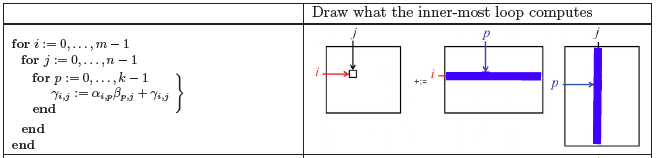
¶Consider again a simple algorithm for computing \(C := A B + C \text{:}\)
Given that we now embrace the convention that \(i \) indexes rows of \(C \) and \(A \text{,}\) \(j \) indexes columns of \(C \) and \(B \text{,}\) and \(p \) indexes "the other dimension," we can call this the IJP ordering of the loops around the assignment statement.
Different orders in which the elements of \(C \) are updated, and the order in which terms of
are added to \(\gamma_{i,j} \text{,}\) are mathematically equivalent as long as each
is performed exactly once. That is, in exact arithmetic, the result does not change. (Computation is typically performed in floating point arithmetic, in which case roundoff error may accumulate slightly differently, depending on the order of the loops. One tends to ignore this when implementing matrix-matrix multiplication.) A consequence is that the three loops can be reordered without changing the result.
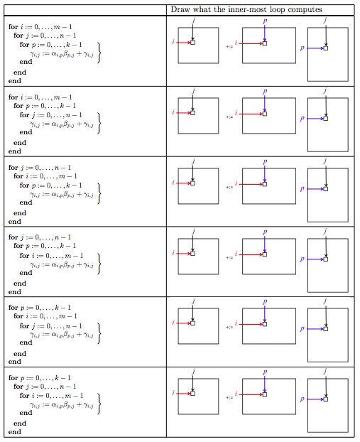
Homework 1.2.4.1.
The IJP ordering is one possible ordering of the loops. How many distinct reorderings of those loops are there?
There are three choices for the outer-most loop: \(i \text{,}\) \(j \text{,}\) or \(p \text{.}\)
Once a choice is made for the outer-most loop, there are two choices left for the second loop.
Once that choice is made, there is only one choice left for the inner-most loop.
Thus, there are \(3! = 3 \times 2 \times 1 = 6 \) loop orderings.
Homework 1.2.4.2.
In directory Assignments/Week1/C make copies of Assignments/Week1/C/Gemm_IJP.c into files with names that reflect the different loop orderings (Gemm_IPJ.c, etc.). Next, make the necessary changes to the loops in each file to reflect the ordering encoded in its name. Test the implementions by executing
make IPJ
make JIP
   ...
for each of the implementations and view the resulting performance by making the indicated changes to the Live Script in
Assignments/Week1/C/data/Plot_All_Orderings.mlx (Alternatively, use the script in Assignments/Week1/C/data/Plot_All_Orderings_m.m). If you have implemented them all, you can test them all by executing make All_Orderings
Homework 1.2.4.3.
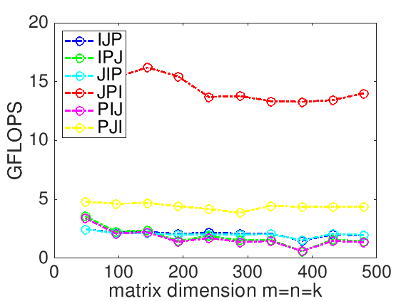
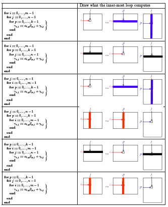
In Figure 1.2.5, the results of Homework 1.2.4.2 on Robert's laptop are reported. What do the two loop orderings that result in the best performances have in common? You may want to use the following worksheet to answer this question:
Homework 1.2.4.4.
In Homework 1.2.4.3, why do they get better performance?
Homework 1.2.4.5.
In Homework 1.2.4.3, why does the implementation that gets the best performance outperform the one that gets the next to best performance?
Think about how and what data get reused for each of the two implementations.
For both the JPI and PJI loop orderings, the inner loop accesses columns of \(C \) and \(A \text{.}\) However,
Each execution of the inner loop of the JPI ordering updates the same column of \(C \text{.}\)
Each execution of the inner loop of the PJI ordering updates a different column of \(C \text{.}\)
In Week 2 you will learn about cache memory. The JPI ordering can keep the column of \(C \) in cache memory, reducing the number of times elements of \(C \) need to be read and written.
If this isn't obvious to you, it should become clearer in the next unit and the next week.
Remark 1.2.7.
One thing that is obvious from all the exercises so far is that the gcc compiler doesn't do a very good job of automatically reordering loops to improve performance, at least not for the way we are writing the code.