PfHP Simple blocking for registers

Unit 2.3.2 Simple blocking for registers

Let's first consider blocking \(C \text{,}\) \(A \text{,}\) and \(B \) into \(4 \times 4 \) submatrices. If we store all three submatrices in registers, then \(3 \times 4 \times 4 = 48 \) doubles are stored in registers.

Remark 2.3.2.

Yes, we are not using all registers (since we assume registers can hold 64 doubles). We'll get to that later.

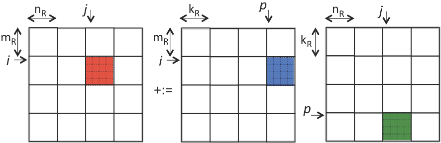
Let us call the routine that computes with three blocks "the kernel". Now the blocked algorithm is a triple-nested loop around a call to this kernel, as captured by the following triple-nested loop

\begin{equation*} \begin{array}{l} {\bf for~} j := 0, \ldots , N-1 \\ ~~~ {\bf for~} i := 0, \ldots , M-1 \\ ~~~ ~~~ {\bf for~} p := 0, \ldots , K-1 \\ ~~~ ~~~ ~~~ {\rm Load~} C_{i,j} , A_{i,p} , {\rm ~and~} B_{p,j} {\rm ~into~registers} \\ ~~~ ~~~ ~~~ C_{i,j} := A_{i,p} B_{p,j} + C_{i,j} \\ ~~~ ~~~ ~~~ {\rm Store~} C_{i,j} {\rm ~to~memory} \\ ~~~ ~~~ {\bf end} \\ ~~~ {\bf end} \\ {\bf end} \end{array} \end{equation*}

and illustrated by

where we use the subscript "R" to indicate it is a block size that targets registers.

Remark 2.3.3.

For our discussion, it is important to order the \(p \) loop last. Next week, it will become even more important to order loops around the kernel in a specific order. We are picking the JIP order here in preparation for that. If you feel like it, you can play with the IJP order (around the kernel) to see how it compares.

The time required to execute this algorithm under our model is given by

\begin{equation*} \begin{array}{l} \begin{array}[t]{c} \underbrace{M N K}\\ \mbox{numb.}\\ \mbox{of MMM}\\ \mbox{with blocks} \end{array} \left( \begin{array}[t]{c} \underbrace{ (m_R n_R + m_R k_R + k_R n_R) \beta_{R \leftrightarrow M} }\\ \mbox{Load blocks of }A, B, \mbox{ and }C \end{array} + \begin{array}[t]{c} \underbrace{ 2 m_R n_R k_R \gamma_R } \\ \mbox{multiplication}\\ \mbox{with blocks} \end{array} + \begin{array}[t]{c} \underbrace{ m_R n_R \beta_{R \leftrightarrow M} }\\ \mbox{Write block of }C \end{array} \right)\\ ~~~=~~~~ \lt \mbox{rearrange} \gt \\ \begin{array}{rcl} 2 (M m_R) (Nn_R)(K k_R) \gamma_R \amp+\amp 2 (M m_R) (N n_R ) K \beta_{R \leftrightarrow M} \\ \amp+\amp (M m_R) N ( K k_R ) \beta_{R \leftrightarrow M} + M (N n_R) ( K k_R ) \beta_{R \leftrightarrow M} \end{array} \\ ~~~=~~~~ \lt \mbox{simplify, distribute, commute, etc.} \gt \\ \begin{array}[t]{c} \underbrace{ 2 m n k \gamma_R}\\ \mbox{useful computation} \end{array} +~~~~~~~ \begin{array}[t]{c} \underbrace{ m n k ( \frac{2}{k_R} + \frac{1}{n_R} + \frac{1}{m_R} ) \beta_{R \leftrightarrow M},} \\ \mbox{overhead} \end{array} \end{array} \end{equation*}

since \(M = m/m_R\) , \(N = n/n_R \text{,}\) and \(K = k/k_R \text{.}\) (Here we assume that \(m \text{,}\) \(n \text{,}\) and \(k \) are integer multiples of \(m_R \text{,}\) \(n_R \text{,}\) and \(k_R \text{.}\))

Remark 2.3.4.

The time spent in computation,

\begin{equation*} 2 m n k \gamma_R, \end{equation*}

is useful time and the time spent in loading and storing data,

\begin{equation*} m n k ( \frac{2}{k_R} + \frac{1}{n_R} + \frac{1}{m_R} ) \beta_{R \leftrightarrow M}, \end{equation*}

is overhead.

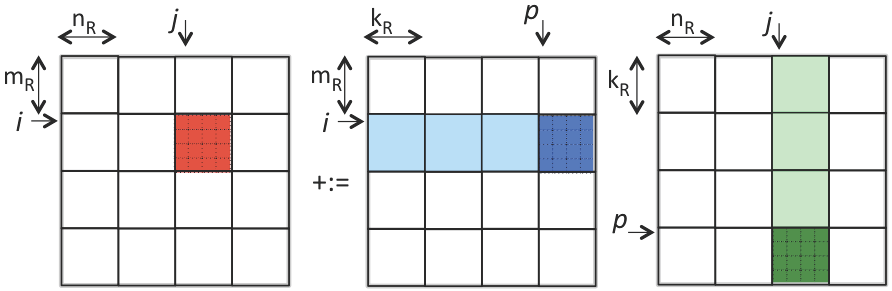
Next, we recognize that since the loop indexed with \(p\) is the inner-most loop, the loading and storing of \(C_{i,j} \) does not need to happen before every call to the kernel, yielding the algorithm

\begin{equation*} \begin{array}{l} {\bf for~} i := 0, \ldots , M-1 \\ ~~~ {\bf for~} j := 0, \ldots , N-1 \\ ~~~ ~~~ {\rm Load~} C_{i,j} \mbox{ into registers} \\ ~~~ ~~~ {\bf for~} p := 0, \ldots , K-1 \\ ~~~ ~~~ ~~~ {\rm Load~} A_{i,p} , {\rm ~and~} B_{p,j} \mbox{ into registers} \\ ~~~ ~~~ ~~~ C_{i,j} := A_{i,p} B_{p,j} + C_{i,j} \\ ~~~ ~~~ {\bf end} \\ ~~~ ~~~ {\rm Store~} C_{i,j} \mbox{ to memory} \\ ~~~ {\bf end} \\ {\bf end} \end{array} \end{equation*}

as illustrated by

Homework 2.3.2.1.

In detail explain the estimated cost of this modified algorithm.

Solution

\begin{equation*} \begin{array}{l} M N K ( 2 m_R n_R k_R ) \gamma_R + \left[ M N ( 2 m_R n_R ) + M N K (m_R k_R + k_R n_R )\right] \beta_{R \leftrightarrow M}\\ ~~~= 2 m n k \gamma_R+ \left[ 2 m n + m n k ( \frac{1}{n_R} + \frac{1}{m_R} ) \right] \beta_{R \leftrightarrow M}. \end{array} \end{equation*}

Here

\(2 m n k \gamma_R \) is time spent in useful computation.
\(\left[ 2 m n + m n k ( \frac{1}{n_R} + \frac{1}{m_R} ) \right] \beta_{R \leftrightarrow M} \) is time spent moving data around, which is overhead.

Homework 2.3.2.2.

In directory Assignments/Week2/C copy the file Assignments/Week2/C/Gemm_JIP_PJI.c into Gemm_JI_PJI.c and combine the loops indexed by P, in the process "removing" it from MyGemm. Think carefully about how the call to Gemm_PJI needs to be changed:

What is the matrix-matrix multiplication that will now be performed by Gemm_PJI?
How do you express that in terms of the parameters that are passed to that routine?

(Don't worry about trying to pick the best block size. We'll get to that later.)

You can test the result by executing

make JI_PJI

View the performance by making the appropriate changes to Assignments/Week2/C/data/Plot_Blocked_MMM.mlx.

Solution

Assignments/Week2/Answers/Gemm_JI_PJI.c

This is the performance on Robert's laptop, with MB=NB=KB=100:

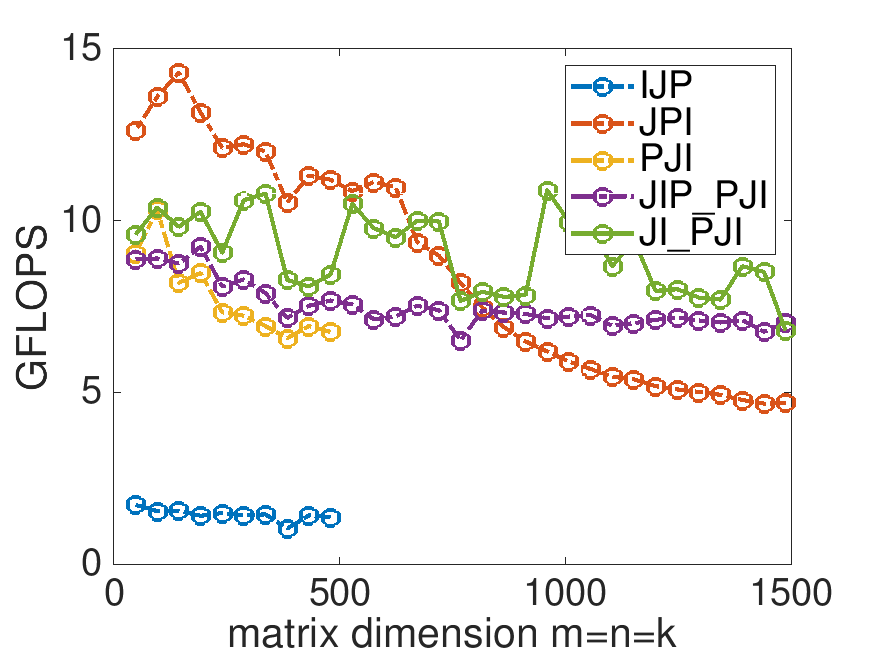
The performance you observe may not really be an improvement relative to Gemm_JIP_PJI.c. What we observe here may be due to variation in the conditions under which the performance was measured.