We postulate that one should never start by considering how to decompose the matrix. Rather, one should start by considering how to decompose the physical problem to be solved. Notice that it is the elements of vectors that are typically associated with data of physical significance and it is therefore their distribution to nodes that is directly related to the distribution of the problem to be solved. A matrix (discretized operator) merely represents the relation between two vectors (discretized spaces):
Since it is more natural to start with distributing the problem to nodes, we partition x and y , and assign portions of these vectors to nodes. The matrix A should then be distributed to nodes in a fashion consistent with the distribution of the vectors, as we shall show next. We will call a matrix distribution physically based if the layout of the vectors which induce the distribution of A to nodes is consistent with where an application would naturally want them. We will use the abbreviation PBMD for Physically Based Matrix Distribution.
As discussed, we must start by describing the distribution of
the vectors, x and y , to nodes, after which
we will show how the matrix distribution is induced
(derived) by the vector distribution.
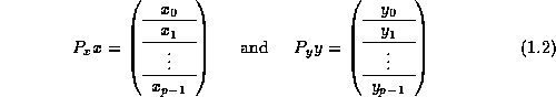
Let ![]() and
and ![]() be permutations so that
be permutations so that
Here ![]() and
and ![]() are the permutations that order the elements of
x and y , respectively,
that are to be assigned to the first node first,
then the ones assigned to the second node, and so forth.
Thus if the nodes are labeled
are the permutations that order the elements of
x and y , respectively,
that are to be assigned to the first node first,
then the ones assigned to the second node, and so forth.
Thus if the nodes are labeled ![]() ,
,
![]() and
and ![]() are assigned to
are assigned to ![]() .
Notice that the above discussion links the linear algebra
object ``vector'' to a mapping to the nodes.
In most other approaches to matrix distribution, vectors
appear as special cases of matrices, or as somehow linked
to the rows and columns of matrices, after the distribution
of matrices is already specified.
We will also link rows and columns of matrices to vectors,
but only after the distribution of the vectors has
been determined, as prescribed by the application.
We again emphasize that this
means we inherently start with the (discretized) physical problem,
rather than the (discretized) operator.
.
Notice that the above discussion links the linear algebra
object ``vector'' to a mapping to the nodes.
In most other approaches to matrix distribution, vectors
appear as special cases of matrices, or as somehow linked
to the rows and columns of matrices, after the distribution
of matrices is already specified.
We will also link rows and columns of matrices to vectors,
but only after the distribution of the vectors has
been determined, as prescribed by the application.
We again emphasize that this
means we inherently start with the (discretized) physical problem,
rather than the (discretized) operator.
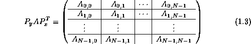
Next, we partition matrix A conformally:
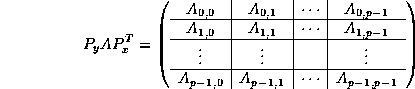
Notice that
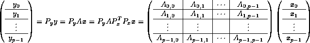
and thus
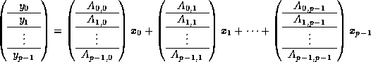
This exposes a natural tie between
sub-vectors of ![]() and corresponding blocks of columns of
and corresponding blocks of columns of ![]() .
.
Also
![]()
so
there is a natural tie between
sub-vectors of ![]() and corresponding blocks of rows of
and corresponding blocks of rows of ![]() .
.
It has been well documented [, ] that for
scalability reasons, it is often important to assign matrices to nodes
of a distributed memory architecture using a so-called
two-dimensional
matrix distribution.
To do so, the p = rc nodes are viewed as a logical
![]() mesh,
mesh,
![]() , with
, with ![]() and
and
![]() . This requires us to decide how
to distribute the sub-vectors to the two-dimensional mesh.
We will assume this is done in column-major order.
(Notice that by appropriate choice of
. This requires us to decide how
to distribute the sub-vectors to the two-dimensional mesh.
We will assume this is done in column-major order.
(Notice that by appropriate choice of ![]() and
and ![]() , this
can always be enforced.)
The distribution of A is now
induced by requiring block of columns
, this
can always be enforced.)
The distribution of A is now
induced by requiring block of columns ![]() to be assigned to the same column of nodes
as sub-vector
to be assigned to the same column of nodes
as sub-vector ![]() , and block of rows
, and block of rows ![]() to the same
row of nodes as sub-vector
to the same
row of nodes as sub-vector ![]() (and thus
(and thus ![]() ).
This is illustrated in
Figure 1.1.
).
This is illustrated in
Figure 1.1.
Often, for load balancing reasons, it becomes important to over-decompose the vectors and matrices, and wrap the sub-blocks onto the node mesh. This can be described by now partitioning x and y so that
where N >> p . Partitioning A conformally yields the blocked matrix
An explicitly
two-dimensional wrapped distribution for the matrix
can now be obtained by
wrapping the blocks of x and y , which induces
a wrapping in the distribution of A , as illustrated
in
Figure 1.2.
Again, the sub-vectors are assigned to the node mesh in column-major
order, wrapping as necessary.
As before, the distribution of A is now
induced by requiring block of columns ![]() to be assigned to the same column of nodes
as sub-vector
to be assigned to the same column of nodes
as sub-vector ![]() , and block or rows
, and block or rows ![]() to the same
row of nodes as sub-vector
to the same
row of nodes as sub-vector ![]() (and thus
(and thus ![]() ).
This is also illustrated in
Figure 1.2.
Notice that the wrapping of the vectors induces a tight wrapping
of blocks of rows of
).
This is also illustrated in
Figure 1.2.
Notice that the wrapping of the vectors induces a tight wrapping
of blocks of rows of ![]() , and a looser wrapping (by a factor of r ) of the
blocks of columns of
, and a looser wrapping (by a factor of r ) of the
blocks of columns of ![]() .
.
We emphasize that the distributions described in
Figures
1.1
and
1.2
may appear to be special cases
of Physically Based Matrix Distribution, since
corresponding sub-blocks of x and y are assigned to the
same node. Notice that by choosing ![]() in Equation 1.2,
a general distribution can be attained [].
in Equation 1.2,
a general distribution can be attained [].
Having just stated that we can achieve total generality, we need to also clearly state that in the initial implementation of PLAPACK, we actually only implement a special case: