2 Cholesky Factorization

  In this section, we discuss the computation of the Cholesky factorization $$A = L L^T$$where A is an $n \times n$ symmetric positive definite matrix and L is an $n \times n$ lowertriangular matrix.

2.1 Basic algorithm

The right-looking algorithm for implementing this operation can be described by partitioning the matrices $$A = \left( \begin{array} { c \vert c } \alpha_{11} & \star \... ... \lambda_{11} & 0 \\ \hline l_{21} & L_{22}\end{array} \right)$$where $\alpha_{11}$ and $\lambda_{11}$ are scalars. As a result, $a_{21}$ and $l_{21}$ are vectors of length n-1 , and $A_{22}$ and $L_{22}$ are matrices of size $(n-1) \times (n-1)$.The $\star$ indicates the symmetric part of A , which will not be updated. Now, $$\begin{eqnarray*} A = \left( \begin{array} { c \vert c } a_{11} & \star \\ \hli... ...11} l_{21} & l_{21} l_{21}^T + L_{22} L_{22}^T\end{array} \right)\end{eqnarray*}$$From this we derive the equations $$\begin{eqnarray*} \lambda_{11} & = & \sqrt{\alpha_{11}} \\ l_{21} & = & a_{21} / \lambda_{11} \\ A_{22} - l_{21} l_{21}^T &=& L_{22} L_{22}^T\end{eqnarray*}$$An algorithm for computing the Cholesky factorization is now given by

1.

Partition $A = \left( \begin{array} { c \vert c } \alpha_{11} & \star \\ \hline a_{21} & A_{22}\end{array} \right)$

2.

$\alpha_{11} \leftarrow \lambda_{11} = \sqrt{ \alpha_{11} }$

3.

$a_{21} \leftarrow l_{21} = a_{21} / \lambda_{11}$

4.

$A_{22} \leftarrow A_{22} - l_{21} l_{21}^T$

5.

continue recursively with $A_{22}$

Note that only the upper or lower triangular part of a symmetric matrix needs to be stored, and the above algorithm only updates the lower portion of the matrix with the result L . As a result, in the step $A_{22} \leftarrow A_{22} - l_{21} l_{21}^T$only the lower portion of $A_{22}$ is updated, which is typically referred to as a symmetric rank-1 update.

One question that may be asked about the above algorithm is what is stored in the matrix after k steps. We answer this by partitioning $$\begin{eqnarray*} A = \left( \begin{array} { c \vert c } A_{TL} & \star \\ \hli... ...vert c } L_{TL} & 0 \\ \hline L_{BL} & L_{BR}\end{array} \right)\end{eqnarray*}$$where $A_{TL}$ and $L_{TL}$ are $k\times k$.Here ``TL '' , ``BL '', and ``BR '' stand for ``Top-Left'', ``Bottom-Left'', and ``Bottom-Right'', respectively. As seen before $$\begin{eqnarray*} A = \left( \begin{array} { c \vert c } A_{TL} & \star \\ \hli... ...} L_{TL}^T & L_{BL} L_{BL}^T + L_{BR} L_{BR}^T\end{array} \right)\end{eqnarray*}$$so that $$\begin{eqnarray*} A_{TL} & = & L_{TL} L_{TL}^T \\ A_{BL} & = & L_{BL} L_{TL}^T \\ A_{BR} &=& L_{BR} L_{BR}^T + L_{BL} L_{BL}^T\end{eqnarray*}$$It can be easily verified that the above algorithm has the effect that after k steps

• $A_{TL}$ has been overwritten by $L_{TL}$,
• $A_{BL}$ has been overwritten by $L_{BL}$,and
• $A_{BR}$ has been overwritten by $A_{BR} - L_{BL} L_{BL}^T$.

Thus, the matrix with which the algorithm is continued at each step is the submatrix $A_{BR}$and to complete the Cholesky factorization, it suffices to compute the factorization of the updated $A_{BR}$.This motivates the algorithm given on the left in Fig. 1.

2.2 Blocked algorithm

The bulk of the computation in the above algorithm is in the symmetric rank-1 update, which performs $O( n^2 )$ operations on $O( n^2 )$ data. It is this ratio of computation to data volume (requiring memory accesses) that stands in the way of high performance. To overcome this, we now show how to reformulate the algorithm in terms of matrix-matrix multiplication (or rank-k updates) which have a more favorable computation to data volume ratio, allowing for more effective use of a microprocessor's cache memory.

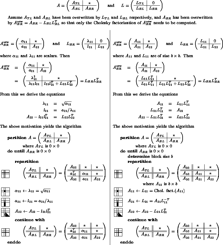
Given the derivation of the basic algorithm given above, it is not difficult to derive a blocked (matrix-matrix operation based) algorithm, as is shown in Fig. 1.

   Figure 1: Similarity in the derivation of a Level-2 (left) and Level-3 (right) BLAS based right-looking Cholesky factorization.

2.3 PLAPACK implementation

  In PLAPACK, information (e.g. size and distribution) regarding a linear algebra object (e.g. matrix or vector) is encoded in a data structure (opaque object) much like MPI encodes communicators. Thus, the calling the calling sequence for a Cholesky factorization need only have one parameter, the object that describes the matrix. One advantage of this approach is that references into the same data can be created as new objects, called views. PLAPACK provides routines that query information associated with an object and other routines that create views. Finally, parallelizing the above blocked algorithm in essense comes down to parallelizing the different major operations:

• Cholesky factorization of $A_{11}$

  $A_{11} \leftarrow L_{11} = \mbox{Chol. fact}(A_{11})$

• Update of $A_{21}$

  $A_{21} \leftarrow L_{21} = A_{21}L_{11}^{-T}$ (solved as triangular solve with multiple-right-hand-sides $L_{11} L_{21}^T = A_{21}^T$)

• Symmetric rank-k update of $A_{22}$

  $A_{22} \leftarrow A_{22} - L_{21} L_{21}^T$

PLAPACK provides parallel kernels that perform these operations.

Basic parallel implementation

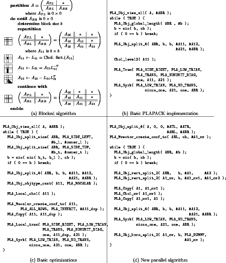
Fig. 2 (a)-(b) illustrate how the developed algorithm is translated into a PLAPACK code. It suffices to know that object A references the original matrix to be factored. Object ABR is a view into the current part of the matrix that still needs to be factored ($A_{BR}$ in previous discussion). The remainder of the code is self explanatory when compared to the algorithm in (a) of that figure. Note that the call to Chol_level2 is a call to a basic (nonblocked) implementation of the Cholesky factorization. That routine itself resembles the presented code in (b) closely.

   Figure 2: Various versions of level-3 BLAS based Cholesky factorization using PLAPACK.

Basic optimizations

While the code presented in Fig. 2 (b) is a straight forward translation of the developed algorithm, it does not provide high performance. The primary reason for this is that the factorization of $A_{11}$ is being performed as a call to a parallel matrix-vector based routine, which requires an extremely large number of communications. These communications can be avoided by choosing the size of $A_{11}$ so that it exists entirely on one node.

In Fig. 2 (c) we show how minor modifications to the PLAPACK implementation in (b) allows us to force $A_{11}$to exist on one node. To understand the optimizations, one must have a rudimentary understanding of how matrices are distributed by PLAPACK. A given matrix A is partitioned like $$A = \left( \begin{array} { c \vert c \vert c } A_{0,0} & \cd... ...\hline A_{(M-1),0} & \cdots & A_{(M-1),(N-1)}\end{array}\right)$$For understanding the code, the sizes of the blocks are not important. What is important is that these blocks are assigned to an $r \times c$ logical mesh of nodes using a two-dimensional cartesian distribution:

• All blocks in the same row of blocks, $A_{i,*}$ are assigned to the same row of nodes.
• All blocks in the same column of blocks, $A_{*,j}$ are assigned to the same column of nodes.

.

Given that the currently active submatrix $A_{BR}$ is distributed to a given logical mesh of nodes, determining a block size so that $A_{11}$ resides on one node requires us to take the minimum of

• the number of columns that can be split off from the left of $A_{BR}$ while remaining in the same block of columns of $A_{BR}$, and
• the number of rows that can be split off from the top of $A_{BR}$ while remaining in the same block of rows of $A_{BR}$.

Once it is guaranteed that $A_{11}$ resides within one node, the call to Chol_level2 can be replaced by a sequential factorization provided by PLA_Local_chol.

Notice that if $A_{11}$ exists within one node, then $A_{21}$ exists within one column of nodes. Recognizing that $A_{21} \leftarrow L_{21} = A_{21} L_{11}^{-T}$is a row-wise operation and thus parallelizes trivially if $L_{11}$ is duplicated within the column that owns $L_{11}$ (and thus $A_{21}$), a further optimization is attained by duplicating $L_{11}$ within the appropriate column of nodes, and performing the update of $A_{21}$locally on those nodes. The resulting PLAPACK code is given in Fig. 2 (c).

A new parallel algorithm

To understand further optimizations, one once again needs to know more about some of the principles underlying PLAPACK. Unlike ScaLAPACK, PLAPACK has a distinct approach to distributing vectors. For scalability reasons, parallel dense linear algebra algorithms must be implemented using a logical two-dimensional mesh of nodes [5,11,13,15]. However, for the distribution of vectors, that two-dimensional mesh is linearized by ordering the nodes in column-major order. Assignment of a vector to the nodes is then accomplished by partitioning the vector in blocks and wrapping these blocks onto the linear array of nodes in round-robin fashion. Assignment of matrices is then dictated by the following principle:

• the i th row of the matrix is assigned to the same row of nodes as the i th element of the vector.
• the j th column of the matrix is assigned to the same column of nodes as the j th element of the vector.

In [8,16] we call this approach to generating a matrix distribution from a vector distribution physically based matrix distribution. A consequence of this assignment strategy is that a column of a matrix can be redistributed like a vector by scattering the elements appropriately within rows of nodes. Similarly, a row of a matrix can be redistributed like a vector by scattering the elements appropriately within columns of nodes. Naturally, redistributing a vector like a column or row of a matrix can be accomplished by reversing these communications.

Note that as a consequence of the last optimization, all computation required to factor $A_{11}$ and update $A_{21}$ is performed within one column of nodes. This is an operation that is very much in the critical path, and thus contributes considerably to the overall time required for the Cholesky factorization. If one views the panel of the matrix $$\left( \begin{array} {c} A_{11} \\ \hline A_{21} \end{array}\right)$$as a collection (panel) of columns, then by simultaneously scattering the elements of these columns of matrices within rows of nodes one can redistribute the panel as a collection of vectors (multivector). Subsequently, $A_{11}$ can be factored as a multivector and, more importantly, considerably more parallelism can be attained during the update of $A_{21}$, since the multivector is distributed to nodes using a one-dimensional data distribution.

It should be noted that the volume of data communicated when redistributing (scattering or gathering) a panel of length n and width b is $O( \frac{n}{r}b )$, where r equals the number of rows in the mesh of nodes. The cost of (parallel) computation subsequently performed on the panel is $O( \frac{n}{r}{b^2})$.Thus, if the block size b is relatively large, there is an advantage to redistributing the panel. Furthermore, the multivector distribution is a natural intermediate distribution for the data movement that subsequently must be performed to duplicate the data as part of the parallel symmetric rank-k update [16]. A further optimization of the parallel Cholesky factorization, for which we do not present code in Fig. 2, takes advantage of this fact.

Naturally, one may get the impression that we have merely hidden all complexity and ugliness in routines like PLA_Chol_mv. Actually, each of those routines themselves are coded at the same high level, and are not substantially more complex than the examples presented.