Subsection 2.2.6 Change of orthonormal basis
¶Homework 2.2.6.1.
Consider the vector \(x = \left( \begin{array}{r} -2 \\ 1 \end{array} \right)\) and the following picture that depicts a rotated basis with basis vectors \(u_0 \) and \(u_1 \text{.}\)
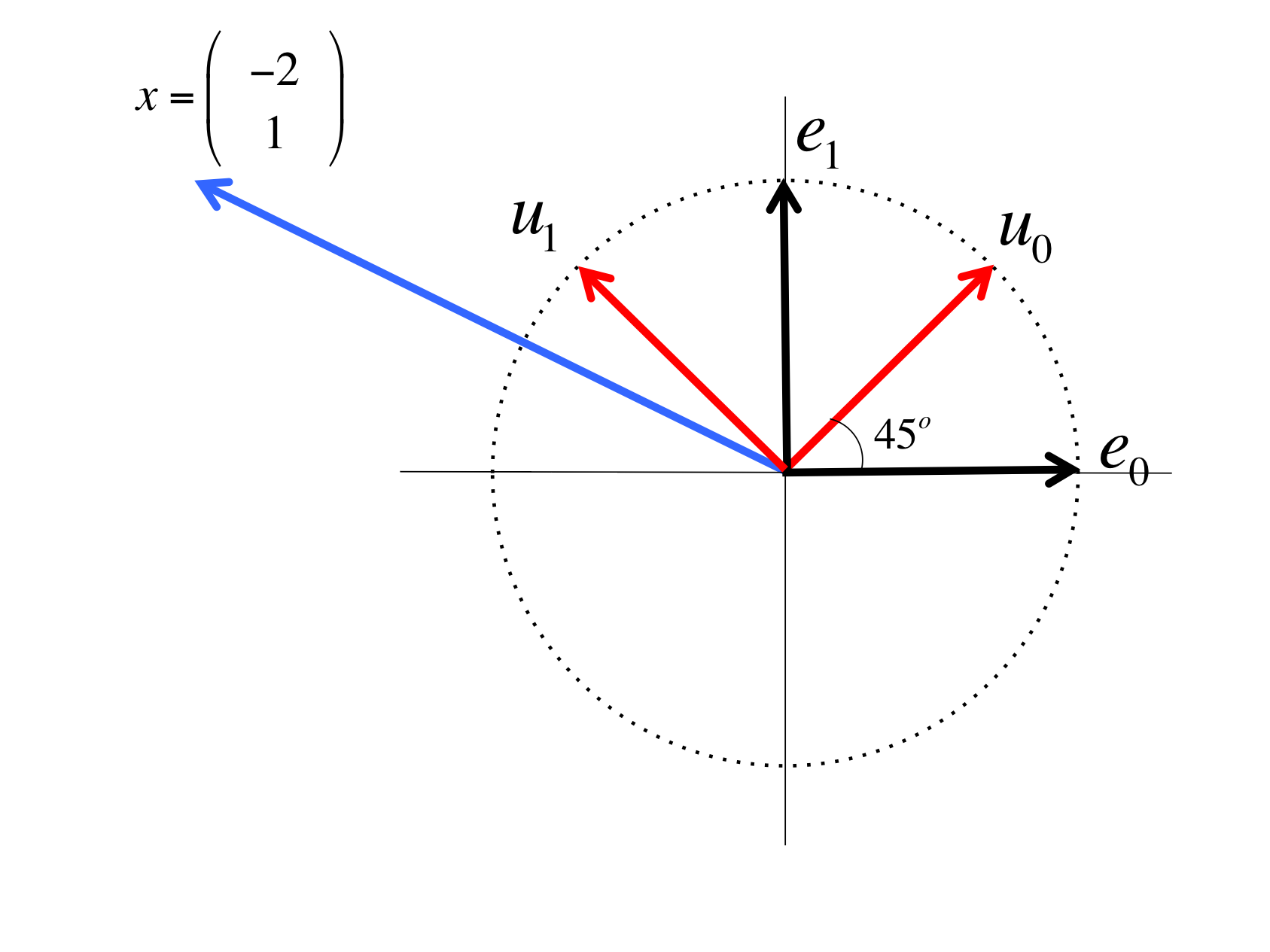
There are a number of approaches to this. One way is to try to remember the formula you may have learned in a pre-calculus course about change of coordinates. Let's instead start by recognizing (from geometry or by applying the Pythagorean Theorem) that
Here are two ways in which you can employ what you have discovered in this course:
-
Since \(u_0 \) and \(u_1 \) are orthonormal vectors, you know that
\begin{equation*} \begin{array}{l} x \\ ~~~=~~~~ \lt u_0 \mbox{ and } u_1 \mbox{ are orthonormal } \gt \\ \begin{array}[t]{c} \underbrace{ ( u_0^T x ) u_0 }\\ \mbox{ component in the } \\ \mbox{ direction of } u_0 \end{array} + \begin{array}[t]{c} \underbrace{ ( u_1^T x ) u_1 }\\ \mbox{ component in the } \\ \mbox{ direction of } u_1 \end{array} \\ ~~~=~~~~ \lt \mbox{ instantiate } u_0 \mbox{ and } u_1 \gt \\ \left( \frac{\sqrt{2}}{2} \left( \begin{array}{c} 1 \\ 1 \end{array} \right)^T \left( \begin{array}{c} -2 \\ 1 \end{array} \right) \right) u_0 + \left( \frac{\sqrt{2}}{2} \left( \begin{array}{c} -1 \\ 1 \end{array} \right)^T \left( \begin{array}{c} -2 \\ 1 \end{array} \right) \right) u_1\\ ~~~ = ~~~~ \lt \mbox{ evaluate } \gt \\ - \frac{\sqrt{2}}{2} u_0 + \frac{3\sqrt{2}}{2} u_1. \end{array} \end{equation*} -
An alternative way to arrive at the same answer that provides more insight. Let \(U = \left( \begin{array}{c | c} u_0 \amp u_1 \end{array} \right) \text{.}\) Then
\begin{equation*} \begin{array}{l} x \\ ~~~ = ~~~~ \lt U \mbox{ is unitary (or orthogonal since it is real valued)} \gt \\ U U^T x \\ ~~~ = ~~~~ \lt \mbox{ instantiate } U \gt \\ \left( \begin{array}{c | c} u_0 \amp u_1 \end{array} \right) \left( \begin{array}{c} u_0^T \\ \hline u_1^T \end{array} \right) x \\ ~~~ = ~~~~ \lt \mbox{ matrix-vector multiplication } \gt \\ \left( \begin{array}{c | c} u_0 \amp u_1 \end{array} \right) \left( \begin{array}{c} u_0^T x \\ \hline u_1^T x \end{array} \right) \\ ~~~ = ~~~~ \lt \mbox{ instantiate } \gt \\ \left( \begin{array}{c | c} u_0 \amp u_1 \end{array} \right) \left( \begin{array}{c} \frac{\sqrt{2}}{2} \left( \begin{array}{c}1 \\ 1 \end{array} \right)^T \left( \begin{array}{c} -2 \\ 1 \end{array} \right) \\ \frac{\sqrt{2}}{2} \left( \begin{array}{c}-1 \\ 1 \end{array} \right)^T \left( \begin{array}{c} -2 \\ 1 \end{array} \right) \end{array} \right)\\ ~~~ = ~~~~ \lt \mbox{ evaluate } \gt \\ \left( \begin{array}{c | c} u_0 \amp u_1 \end{array} \right) \left( \begin{array}{c} -\frac{\sqrt{2}}{2} \\ \frac{3 \sqrt{2}}{2} \end{array} \right) \\ ~~~ = ~~~~ \lt \mbox{ simplify } \gt \\ \left( \begin{array}{c | c} u_0 \amp u_1 \end{array} \right) \left( \frac{\sqrt{2}}{2} \left( \begin{array}{c} -1 \\ 3 \end{array} \right) \right) \end{array} \end{equation*}
Below we compare side-by-side how to describe a vector \(x\) using the standard basis vectors \(e_0, \ldots , e_{m-1} \) (on the left) and vectors \(u_0, \ldots , u_{m-1} \) (on the right):
The vector \(x = \left( \begin{array}{c} \chi_0^{\phantom{T}} \\ \vdots \\ \chi_{m-1}^{\phantom{T}} \end{array} \right)\) describes the vector \(x \) in terms of the standard basis vectors \(e_0, \ldots , e_{m-1} \text{:}\)
Illustration: 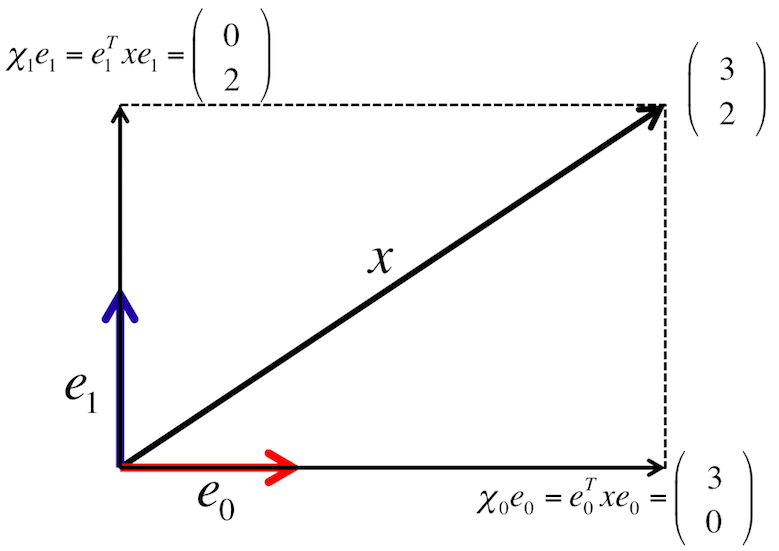
The vector \(\widehat x = \left( \begin{array}{c} u_0^T x \\ \vdots \\ u_{m-1}^T x \end{array} \right)\) describes the vector \(x \) in terms of the orthonormal basis \(u_0, \ldots , u_{m-1} \text{:}\)
Illustration (\(q \) should be \(u\) here): 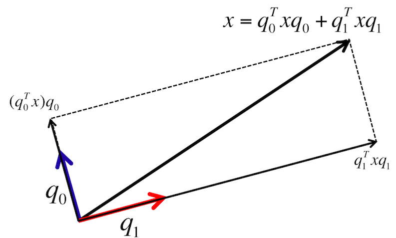
Another way of looking at this is that if \(u_0, u_1, \ldots , u_{m-1}\) is an orthonormal basis for \(\C^m \text{,}\) then any \(x\in \C^m \) can be written as a linear combination of these vectors:
Now,
Thus \(u_i^H x = \alpha_i \text{,}\) the coefficient that multiplies \(u_i \text{.}\)
Remark 2.2.6.1.
The point is that given vector \(x \) and unitary matrix \(U \text{,}\) \(U^H x \) computes the coefficients for the orthonormal basis consisting of the columns of matrix \(U \text{.}\) Unitary matrices allow one to elegantly change between orthonormal bases.