ALAFF Case 1: $A $ has linearly independent columns

🔗

Subsection 4.3.2 Case 1: $A$ has linearly independent columns

fit width

🔗

Let us start by discussing how to use the SVD to find

$\widehat x$ that satisfies

$\begin{equation*} \| b - A \widehat x \|_2 = \min_x \| b - A x \|_2, \end{equation*}$

🔗

for the case where

$A \in \Cmxn$ has linearly independent columns (in other words,

$\rank( A ) = n$ ).

🔗

Let

$A = U_L \Sigma_{TL} V^H$ be its reduced SVD decomposition. (Notice that

$V_L = V$ since

$A$ has linearly independent columns and hence

$V_L$ is

$n \times n$ and equals

$V \text{.}$ )

🔗

Here is a way to find the solution based on what we encountered before: Since

$A$ has linearly independent columns, the solution is given by

$\widehat x = ( A^H A )^{-1} A^H b$ (the solution to the normal equations). Now,

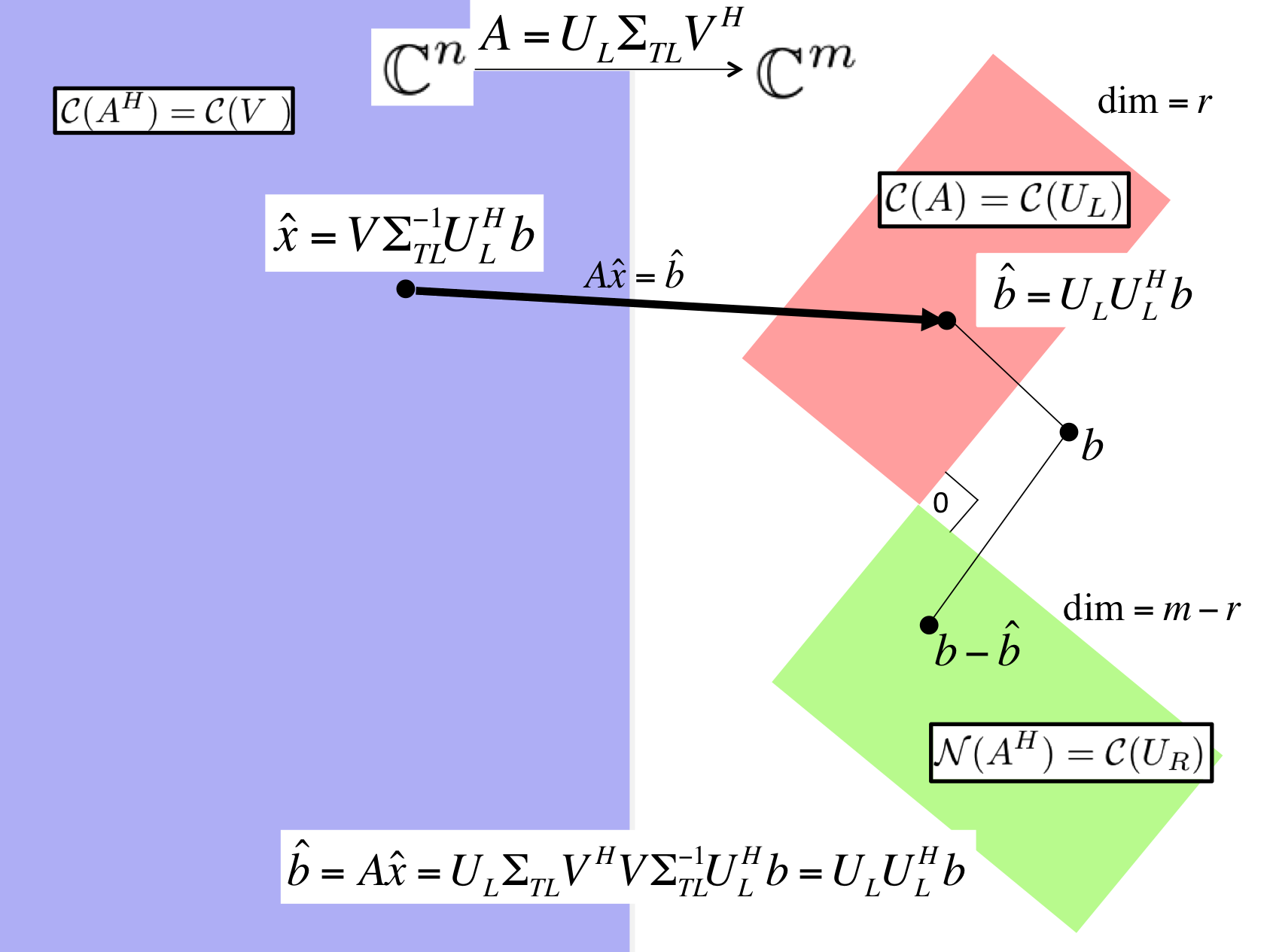
$\begin{equation*} \begin{array}{l} \widehat x \\ ~~~=~~~~ \lt {\rm solution~to~the~normal~equations} \gt \\ ( A^H A )^{-1} A^H b \\ ~~~ = ~~~~ \lt A = U_L \Sigma_{TL} V^H \gt \\ \left[ ( U_L \Sigma_{TL} V^H )^H ( U_L \Sigma_{TL} V^H ) \right]^{-1} ( U_L \Sigma_{TL} V^H )^H b \\ ~~~ = ~~~~ \lt ( B C D )^H = ( D^H C^H B^H) {\rm ~and~} \Sigma_{TL}^H = \Sigma_{TL} \gt \\ \left[ ( V \Sigma_{TL} U_L^H ) ( U_L \Sigma_{TL} V^H ) \right]^{-1} ( V \Sigma_{TL} U_L^H ) b \\ ~~~ = ~~~~ \lt U_L^H U_L = I \gt \\ \left[ V \Sigma_{TL} \Sigma_{TL} V^H \right]^{-1} V \Sigma_{TL} U_L^H b \\ ~~~ = ~~~~ \lt V^{-1} = V^H {\rm ~and~} ( B C D )^{-1} = D^{-1} C^{-1} B^{-1} \gt \\ V \Sigma_{TL}^{-1} \Sigma_{TL}^{-1} V^H V \Sigma_{TL} U_L^H b \\ ~~~ = ~~~~ \lt V^H V = I \mbox{ and } \Sigma_{TL}^{-1} \Sigma_{TL} = I \gt \\ V \Sigma_{TL}^{-1} U_L^H b \end{array} \end{equation*}$

Solving LLS via the SVD when $A$ had linearly independent columns (and hence the row space of $A$ equals $\Cn$ ).

🔗

Alternatively, we can come to the same conclusion without depending on the Method of Normal Equations, in preparation for the more general case discussed in the next subsection. The derivation is captured in Figure 4.3.2.1.

$\begin{equation*} \begin{array}{l} \min_{x \in \Cn} \| b - A x \|_2^2 \\ ~~~=~~~~ \lt \mbox{ substitute the SVD} A = U \Sigma V^H \gt \\ \min_{x \in \Cn} \| b - U \Sigma V^H x \|_2^2 \\ ~~~=~~~~ \lt \mbox{ substitute } I = U U^H \mbox{ and factor out } U \gt \\ \min_{x \in \Cn} \| U ( U^H b - \Sigma V^H x ) \|_2^2 \\ ~~~=~~~~ \lt \mbox{ multiplication by a unitary matrix preserves two-norm } \gt \\ \min_{x \in \Cn} \| U^H b - \Sigma V^H x \|_2^2 \\ ~~~=~~~~ \lt \mbox{ partition, partitioned matrix-matrix multiplication } \gt \\ \min_{x \in \Cn} \left\| \FlaTwoByOne{U_L^H b}{U_R^Hb} - \FlaTwoByOne{\Sigma_{TL}}{0} V^H x \right\|_2^2 \\ ~~~=~~~~ \lt \mbox{ partitioned matrix-matrix multiplication and addition } \gt \\ \min_{x \in \Cn} \left\| \FlaTwoByOne {U_L^H b - \Sigma_{TL} V^H x} {U_R^Hb} \right\|_2^2 \\ ~~~=~~~~ \lt \left\| \left( \begin{array}{c} v_T \\ \hline v_B \end{array} \right) \right\|_2^2 = \| v_T \|_2^2 + \| v_B \|_2^2 \gt \\ \min_{x \in \Cn} \left\| {U_L^H b - \Sigma_{TL} V^H x } \right\|_2^2 + \left\| U_R^H b \right\|_2^2 \end{array} \end{equation*}$

🔗

The

$x$ that solves

$\Sigma_{TL} V^H x = U_L^H b$ minimizes the expression. That

$x$ is given by

$\begin{equation*} \widehat x = V \Sigma_{TL}^{-1} U_L^H b. \end{equation*}$

🔗

since

$\Sigma_{TL}$ is a diagonal matrix with only nonzeroes on its diagonal and

$V$ is unitary.

🔗

Here is yet another way of looking at this: we wish to compute

$\widehat x$ that satisfies

$\begin{equation*} \| b - A \widehat x \|_2 = \min_x \| b - A x \|_2, \end{equation*}$

🔗

for the case where

$A \in \Cmxn$ has linearly independent columns. We know that

$A = U_L \Sigma_{TL} V^H \text{,}$ its Reduced SVD. To find the

$x$ that minimizes, we first project

$b$ onto the column space of

$A \text{.}$ Since the column space of

$A$ is identical to the column space of

$U_L \text{,}$ we can project onto the column space of

$U_L$ instead:

$\begin{equation*} \widehat b = U_L U_L^H b. \end{equation*}$

🔗

(Notice that this is not because

$U_L$ is unitary, since it isn't. It is because the matrix

$U_L U_L^H$ projects onto the columns space of

$U_L$ since

$U_L$ is orthonormal.) Now, we wish to find

$\widehat x$ that exactly solves

$A \widehat x = \widehat b \text{.}$ Substituting in the Reduced SVD, this means that

$\begin{equation*} U_L \Sigma_{TL} V^H \widehat x = U_L U_L^H b. \end{equation*}$

🔗

Multiplying both sides by

$U_L^H$ yields

$\begin{equation*} \Sigma_{TL} V^H \widehat x = U_L^H b. \end{equation*}$

🔗

and hence

$\begin{equation*} \widehat x = V \Sigma_{TL}^{-1} U_L^H b. \end{equation*}$

🔗

We believe this last explanation probably leverages the Reduced SVD in a way that provides the most insight, and it nicely motivates how to find solutions to the LLS problem when

$\rank( A ) \lt r \text{.}$

🔗

The steps for solving the linear least squares problem via the SVD, when

$A \in \Cmxn$ has linearly independent columns, and the costs of those steps are given by

Compute the Reduced SVD $A = U_L \Sigma_{TL} V^H \text{.}$

We will not discuss practical algorithms for computing the SVD until much later. We will see that the cost is $O( m n^2 )$ with a large constant.
Compute $\widehat x = V \Sigma_{TL}^{-1} U_L^H b \text{.}$

The cost of this is approximately,
- Form $y_T = U_L^H b \text{:}$ $2 m n$ flops.
- Scale the individual entries in $y_T$ by dividing by the corresponding singular values: $n$ divides, overwriting $y_T = \Sigma_{TL}^{-1} y_T \text{.}$ The cost of this is negligible.
- Compute $\widehat x = V y_T \text{:}$ $2 n^2$ flops.
The devil is in the details of how the SVD is computed and whether the matrices $U_L$ and/or $V$ are explicitly formed.

Subsection 4.3.2 Case 1: AA has linearly independent columns

Subsection 4.3.2 Case 1: $A$ has linearly independent columns