Unit 3.2.2 Streaming submatrices of \(C \) and \(B \)
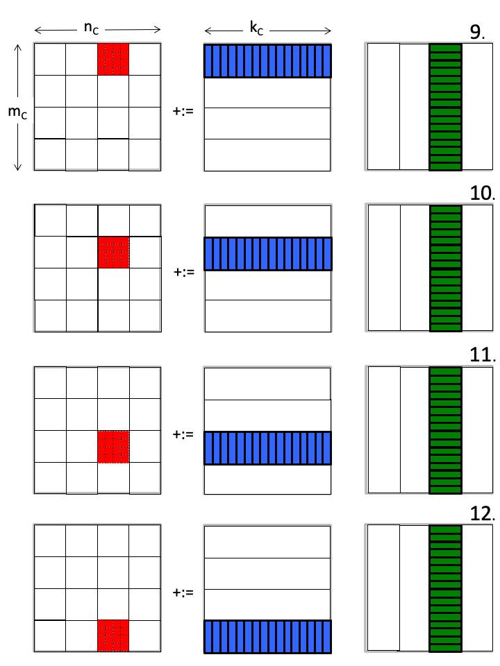
We illustrate the execution of Gemm_JI_4x4Kernel with one set of three submatrices \(C_{i,j} \text{,}\) \(A_{i,p} \text{,}\) and \(B_{p,j} \) in Figure 3.2.4 for the case where \(m_R = n_R = 4 \) and \(m_C = n_C = k_C = 4 \times m_R \text{.}\)
\(J = 0 \)
\(J = 1 \)
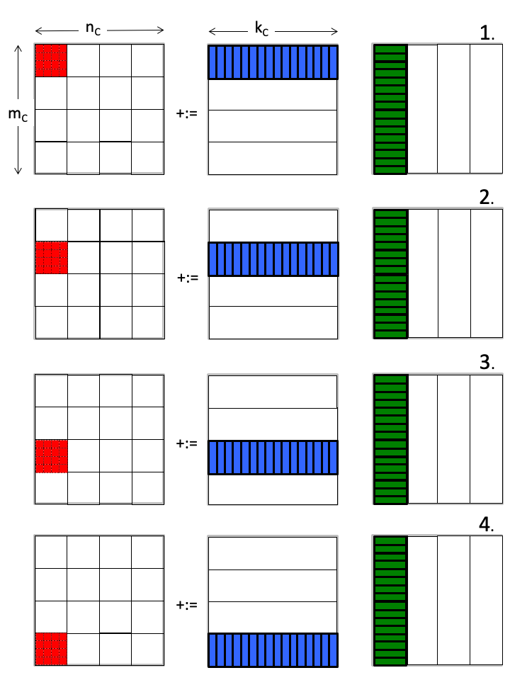

\(J = 2 \)
\(J = 3 \)

Download PowerPoint source for illustration. PDF version.
Notice that
The \(m_R \times n_R \) micro-tile of \(C_{i,j} \) is not reused again once it has been updated. This means that at any given time only one such matrix needs to be in the cache memory (as well as registers).
Similarly, a micro-panel of \(B_{p,j} \) is not reused and hence only one such panel needs to be in cache. It is submatrix \(A_{i,p} \) that must remain in cache during the entire computation.
By not keeping the entire submatrices \(C_{i,j} \) and \(B_{p,j} \) in the cache memory, the size of the submatrix \(A_{i,p} \) can be increased, which can be expected to improve performance. We will refer to this as "streaming" micro-tiles of \(C_{i,j} \) and micro-panels of \(B_{p,j} \text{,}\) while keeping all of block \(A_{i,p} \) in cache.
Remark 3.2.5.
We could have chosen a different order of the loops, and then we may have concluded that submatrix \(B_{p,j} \) needs to stay in cache while streaming a micro-tile of \(C \) and small panels of \(A\text{.}\) Obviously, there is a symmetry here and hence we will just focus on the case where \(A_{i,p} \) is kept in cache.
Homework 3.2.2.1.
Reorder the updates in Figure 3.2.4 so that \(B \) stays in cache while panels of \(A \) are streamed.
You may want to use the PowerPoint source for that figure: Download PowerPoint source.
Answer (referring to the numbers in the top-right corner of each iteration):
Here is the PowerPoint source for one solution: Download PowerPoint source.
The second observation is that now that \(C_{i,j} \) and \(B_{p,j} \) are being streamed, there is no need for those submatrices to be square. Furthermore, for
Gemm_PIJ_JI_12x4Kernel.cand
Gemm_IPJ_JI_12x4Kernel.c,the larger \(n_C \text{,}\) the more effectively the cost of bringing \(A_{i,p} \) into cache is amortized over computation: we should pick \(n_C = n \text{.}\) (Later, we will reintroduce \(n_C \text{.}\)) Another way of thinking about this is that if we choose the PIJ loop around the JI ordering around the micro-kernel (in other words, if we consider the Gemm_PIJ_JI_12x4Kernel implementation), then we notice that the inner loop of PIJ (indexed with J) matches the outer loop of the JI double loop, and hence those two loops can be combined, leaving us with an implementation that is a double loop (PI) around the double loop JI.
Homework 3.2.2.2.
Copy Assignments/Week3/C/Gemm_PIJ_JI_MRxNRKernel.c into Gemm_PI_JI_MRxNRKernel.c and remove the loop indexed with \(j \) from MyGemm, making the appropriate changes to the call to the routine that implements the micro-kernel. Collect performance data by executing
make PI_JI_12x4Kernelin that directory. The resulting performance can be viewed with Live Script
Assignments/Week3/C/data/Plot_XY_JI_MRxNRKernel.mlx.
Assignments/Week3/Answers/Gemm_PI_JI_MRxNRKernel.c.
On Robert's laptop, for \(m_R \times n_R = 12 \times 4 \text{:}\)

By removing that loop, we are simplifying the code without it taking a performance hit.
By combining the two loops we reduce the number of times that the blocks \(A_{i,p} \) need to be read from memory:
which equals
Hence, the ratio of time spent in useful computation, and time spent in moving data between main memory and cache is given by
Another way of viewing this is that the ratio between the number of floating point operations, and number of doubles loaded and stored is given by
If, for simplicity, we take \(m_C = k_C = b \) then we get that
if \(b \) is much smaller than \(n \text{.}\) This is a slight improvement over the analysis from the last unit.
Remark 3.2.6.
In our future discussions, we will use the following terminology:A \(m_R \times n_R \) submatrix of \(C \) that is being updated we will call a micro-tile.
The \(m_R \times k_C \) submatrix of \(A \) and \(k_C \times n_R \) submatrix of \(B \) we will call micro-panels.
The routine that updates a micro-tile by multiplying two micro-panels we will call the micro-kernel.
Remark 3.2.7.
The various block sizes we will further explore are
\(m_R \times n_R \text{:}\) the sizes of the micro-tile of \(C \) that is kept in the registers.
\(m_C \times k_C \text{:}\) the sizes of the block of \(A \) that is kept in the L2 cache.