Matrices are stored in two-dimensional arrays while computer memory is inherently one-dimensional in the way it is addressed. So, we need to agree on how we are going to store matrices in memory.
Figure1.2.1 Mapping of \(m \times n \) matrix \(A \) to memory with column-major order. Obviously, one could use the alternative known as row-major ordering.
Homework1.2.1
Let the following picture represent data stored in memory starting at address A:
Figure1.2.2 Addressing a matrix embedded in an array with \({\tt ldA} \) rows. At the left we illustrate a \(4 \times 3 \) submatrix of a \({\tt ldA} \times 4 \) matrix. In the middle, we illustrate how this is mapped into an linear array {\tt a}. In the right, we show how defining the C macro #define alpha(i,j) A[ (j)*ldA + (i)] allows us to address the matrix in a more natural way.
What we depict there is a matrix that is embedded in a larger matrix. The larger matrix consists of ldA (the leading dimension) rows and some number of columns. If column-major order is used to store the larger matrix, then addressing the elements in the submatrix requires knowledge of the leading dimension of the larger matrix. In the C programming language, if the top-left element of the submatrix is stored at address A, then one can address the \((i,j) \) element as A[ j*ldA + i ]. We typically define a macro that makes addressing the elements more natural:
#define alpha(i,j) A[ (j)*ldA + (i) ]
where we assume that the variable or constant ldA holds the leading dimension parameter.
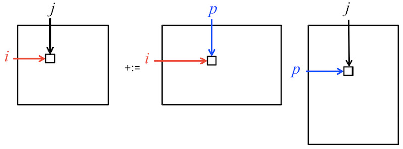
Given that we now embrace the convention that \(i \) indexes rows of \(C \) and \(A \text{,}\) \(j \) indexes columns of \(C \) and \(B \text{,}\) and \(p \) indexes "the other dimension," we can call this the IJP ordering of the loops around the assignment statement.
The order in which the elements of \(C \) are updated, and the order in which terms of
are added to \(\gamma_{i,j} \) is mathematically equivalent. (There would be a possible change in the result due to round-off errors when floating point arithmetic occurs, but this is ignored.) What this means is that the three loops can be reordered without changing the result. That is, in exact arithmetic, the result does not change. However, computation is typically performed in floating point arithmetic, in which case roundoff error may accumulate slightly differently, depending on the order of the loops.
Homework1.2.4
The IJP ordering is one possible ordering of the loops. How many distinct reorderings of those loops are there?
There are three choices for the outer-most loop: \(i \text{,}\) \(j \text{,}\) or \(p \text{.}\) Once a choice is made for the outer-most loop, there are two choices left for the second loop. Once that choice is made, there is only one choice left for the inner-most loop. Thus, there are \(3! = 3 \times 2 \times 1 = 6 \) loop orderings.
Homework1.2.5
In directory Assignments/Week1/C make copies of Assignments/Week1/C/Gemm_IJP.c into files with names that reflect the different loop orderings (Gemm_IPJ.c, etc.). Next, make the necessary changes to the loops in each file to reflect the ordering encoded in its name. Test the implementions by executing
Figure1.2.3 Performance comparison of all different orderings of the loops, on Robert's laptop.
Homework1.2.6
In Figure 1.2.3, the results of Homework 1.2.5 on Robert's laptop are reported. What do the two loop orderings that result in the best performances have in common?
They both have the loop indexed with \(i \) as the inner-most loop.
What is obvious is that ordering the loops matters. Changing the order changes how data in memory are accessed, and that can have a considerable impact on the performance that is achieved. The bottom graph includes a plot of the performance of the reference implementation and scales the y-axis so that the top of the graph represents the theoretical peak of a single core of the processor. What it demonstrates is that there is a lot of room for improvement.