Section 3.3 Contiguous Memory Access is Important
Unit 3.3.1
One would think that once one introduces blocking, the higher performance observed for small matrix sizes will be maintained as the problem size increases. This is not what you observed: there is still a steady decrease in performance. To investigate what is going on, copy the driver routine in driver.c into driver_ldim.c and in that new file change the line
ldA = ldB = ldC = size;to
ldA = ldB = ldC = lastThis sets the leading dimension of matrices \(A\text{,}\) \(B \text{,}\) and \(C \) to the largest problem size to be tested, for all experiments. Collect performance data by executing
make Five_Loops_ldimin that directory. The resulting performance can be viewed with Live Script
Assignments/Week3/C/data/Plot_Five_Loops.mlx.What is going on here? Modern architectures like the Haswell processor have a feature called "hardware prefetching" that speculatively preloads data into caches based on observed access patterns so that this loading is hopefully overlapped with computation. Processors also organize memory in terms of pages, for reasons that go beyond the scope of this course. For our purposes, a page is a contiguous block of memory of 4 Kbytes (4096 bytes or 512 doubles). Prefetching only occurs within a page. Since the leading dimension is now large, when the computation moves from column to column in a matrix data is not prefetched. You may want to learn more on memory pages by visiting https://en.wikipedia.org/wiki/Page_(computer_memory) on Wikipedia.
The bottom line: early in the course we discussed that marching contiguously through memory is a good thing. While we claim that we block for the caches, in practice the data is not contiguous and hence we can't really control how the data is brought into caches and where it exists at a particular time in the computation.
Unit 3.3.2
Homework 3.3.2
In the setting of the five loops, the microkernel updates \(C := A B + C \) where \(C \) is \(m_R \times n_R \text{,}\) \(A \) is \(m_R \times k_C \text{,}\) and \(B\) is \(k_C \times n_R \text{.}\) How many matrix elements of \(C \) have to be brought into registers to perform this computation? How many flops are performed with these elements? How many flops are performed with each element of \(C \text{?}\) We seem to have settled on a \(m_R \times n_R = 12 \times 4 \) microtile. Let's use \(k_C = 128 \text{.}\) What is the ratio for these parameters?
The next step towards optimizing the microkernel recognizes that computing with contiguous data (accessing data with a "stride one" access pattern) improves performance. The fact that the \(m_R \times n_R \) microtile of \(C\) is not in contiguous memory is not particularly important. The cost of bringing it into the vector registers from some layer in the memory is mostly inconsequential because a lot of computation is performed before it is written back out. It is the repeated accessing of the elements of \(A \) and \(B \) that can benefit from stride one access.

Picture adapted from [4].
void PackMicroPanelA_MRxKC( int m, int k, double *A, int ldA, double *Atilde )
/* Pack a micro-panel of A into buffer pointed to by Atilde.
   This is an unoptimized implementation for general MR and KC. */
{
  /* March through A in column-major order, packing into Atilde as we go. */

  if ( m == MR )   /* Full row size micro-panel.*/
    for ( int p=0; p<k; p++ )
      for ( int i=0; i<MR; i++ )
	*Atilde++ = alpha( i, p );
  else /* Not a full row size micro-panel.  We pad with zeroes. */
    for ( int p=0; p<k; p++ ) {
      for ( int i=0; i<m; i++ )
	*Atilde++ = alpha( i, p );
      for ( int i=m; i<MR; i++ )
	*Atilde++ = 0.0;
    }
}

void PackBlockA_MCxKC( int m, int k, double *A, int ldA, double *Atilde )
/* Pack a MC x KC block of A.  MC is assumed to be a multiple of MR.  The block is
   packed into Atilde a micro-panel at a time. If necessary, the last micro-panel
   is padded with rows of zeroes. */
{
  for ( int i=0; i<)m; i+= MR ){
    int ib = min( MR, m-i );
    PackMicroPanelA_MRxKC( ib, k, &alpha( i, 0 ), ldA, Atilde );
    Atilde += ib * k;
  }
}
void PackMicroPanelB_KCxNR( int k, int n, double *B, int ldB, double *Btilde )
/* Pack a micro-panel of B into buffer pointed to by Btilde.
   This is an unoptimized implementation for general KC and NR. */
{
  /* March through B in row-major order, packing into Btilde as we go. */

  if ( n == NR ) /* Full column width micro-panel.*/
    for ( int p=0; p<k; p++ )
      for ( int j=0; j<NR; j++ )
	*Btilde++ = beta( p, j );
  else /* Not a full row size micro-panel.  We pad with zeroes. */
    for ( int p=0; p<k; p++ ) {
      for ( int j=0; j<n; j++ )
	*Btilde++ = beta( p, j );
      for ( int j=n; j<NR; j++ )
	*Btilde++ = 0.0;
    }
}

void PackPanelB_KCxNC( int k, int n, double *B, int ldB, double *Btilde )
/* Pack a KC x NC panel of B.  NC is assumed to be a multiple of NR.  The block is
   packed into Btilde a micro-panel at a time. If necessary, the last micro-panel
   is padded with columns of zeroes. */
{
  for ( int j=0; j<n; j+= NR ){
    int jb = min( NR, n-j );

    PackMicroPanelB_KCxNR( k, jb, &beta( 0, j ), ldB, Btilde );
    Btilde += k * jb;
  }
}
Two successive rank-1 updates of the microtile can be given by
\begin{equation*}
\begin{array}{l}
\left(\begin{array}{c c c c}
\gamma_{0,0} \amp \gamma_{0,1} \amp \gamma_{0,2} \amp \gamma_{0,3} \\
\gamma_{1,0} \amp \gamma_{1,1} \amp \gamma_{1,2} \amp \gamma_{0,3} \\
\gamma_{2,0} \amp \gamma_{2,1} \amp \gamma_{2,2} \amp \gamma_{0,3} \\
\gamma_{3,0} \amp \gamma_{3,1} \amp \gamma_{3,2} \amp \gamma_{0,3}
\end{array}\right)
+:= \\
~~~
\left(\begin{array}{c}
\alpha_{0,p} \\
\alpha_{1,p} \\
\alpha_{2,p} \\
\alpha_{3,p}
\end{array}\right)
\left(\begin{array}{c c c c}
\beta_{p,0} \amp \beta_{p,1} \amp \beta_{p,2} \amp \beta_{p,3}
\end{array} \right)
+
\left(\begin{array}{c}
\alpha_{0,p+1} \\
\alpha_{1,p+1} \\
\alpha_{2,p+1} \\
\alpha_{3,p+1}
\end{array}\right)
\left(\begin{array}{c c c c}
\beta_{p+1,0} \amp \beta_{p+1,1} \amp \beta_{p+1,2} \amp \beta_{p+1,3}
\end{array} \right)
.
\end{array}
\end{equation*}
Since \(A \) and \(B \) are stored with column-major order, the four elements of \(\alpha_{[0:3],p}\) are contiguous in memory, but they are (generally) not contiguously stored with \(\alpha_{[0:3],p+1}\text{.}\) Elements \(\beta_{p,[0:3]} \) are (generally) also not contiguous. The access pattern during the computation by the microkernel would be much more favorable if the \(A \) involved in the microkernel was packed in column-major order with leading dimension \(m_R \text{:}\)


void LoopFive( int m, int n, int k, double *A, int ldA,
double *B, int ldB, double *C, int ldC )
{
for ( int j=0; j<n; j+=NC ) {
int jb = min( NC, n-j ); /* Last loop may not involve a full block */
LoopFour( m, jb, k, A, ldA, &beta( 0,j ), ldB, &gamma( 0,j ), ldC );
}
}
void LoopFour( int m, int n, int k, double *A, int ldA, double *B, int ldB,
double *C, int ldC )
{
double *Btilde = ( double * ) malloc( KC * NC * sizeof( double ) );
for ( int p=0; p<k; p+=KC ) {
int pb = min( KC, k-p ); /* Last loop may not involve a full block */
PackPanelB_KCxNC( pb, n, &beta( p, 0 ), ldB, Btilde );
LoopThree( m, n, pb, &alpha( 0, p ), ldA, Btilde, C, ldC );
}
free( Btilde);
}
void LoopThree( int m, int n, int k, double *A, int ldA, double *Btilde, double *C, int ldC )
{
double *Atilde = ( double * ) malloc( MC * KC * sizeof( double ) );
for ( int i=0; i<m; i+=MC ) {
int ib = min( MC, m-i ); /* Last loop may not involve a full block */
PackBlockA_MCxKC( ib, k, &alpha( i, 0 ), ldA, Atilde );
LoopTwo( ib, n, k, Atilde, Btilde, &gamma( i,0 ), ldC );
}
free( Atilde);
}
void LoopTwo( int m, int n, int k, double *Atilde, double *Btilde, double *C, int ldC )
{
for ( int j=0; j<n; j+=NR ) {
int jb = min( NR, n-j );
LoopOne( m, jb, k, Atilde, &Btilde[ j*k ], &gamma( 0,j ), ldC );
}
}
void LoopOne( int m, int n, int k, double *Atilde, double *MicroPanelB, double *C, int ldC )
{
for ( int i=0; i<m; i+=MR ) {
int ib = min( MR, m-i );
Gemm_4x4Kernel_Packed( k,Ã[ i*k ], MicroPanelB, &gamma( i,0 ), ldC );
}
void Gemm_4x4Kernel_Packed( int k,
		        double *BlockA, double *PanelB, double *C, int ldC )
{
  __m256d gamma_0123_0 = _mm256_loadu_pd( &gamma( 0,0 ) );
  __m256d gamma_0123_1 = _mm256_loadu_pd( &gamma( 0,1 ) );
  __m256d gamma_0123_2 = _mm256_loadu_pd( &gamma( 0,2 ) );
  __m256d gamma_0123_3 = _mm256_loadu_pd( &gamma( 0,3 ) );

  __m256d beta_p_j;

  for ( int p=0; p\lt;k; p++ ){
    /* load alpha( 0:3, p ) */
    __m256d alpha_0123_p = _mm256_loadu_pd( BlockA );

    /* load beta( p, 0 ); update gamma( 0:3, 0 ) */
    beta_p_j = _mm256_broadcast_sd( PanelB );
    gamma_0123_0 = _mm256_fmadd_pd( alpha_0123_p, beta_p_j, gamma_0123_0 );

    /* load beta( p, 1 ); update gamma( 0:3, 1 ) */
    beta_p_j = _mm256_broadcast_sd( PanelB+1 );
    gamma_0123_1 = _mm256_fmadd_pd( alpha_0123_p, beta_p_j, gamma_0123_1 );

    /* load beta( p, 2 ); update gamma( 0:3, 2 ) */
    beta_p_j = _mm256_broadcast_sd( PanelB+2 );
    gamma_0123_2 = _mm256_fmadd_pd( alpha_0123_p, beta_p_j, gamma_0123_2 );

    /* load beta( p, 3 ); update gamma( 0:3, 3 ) */
    beta_p_j = _mm256_broadcast_sd( PanelB+3 );
    gamma_0123_3 = _mm256_fmadd_pd( alpha_0123_p, beta_p_j, gamma_0123_3 );

    BlockA += MR;
    PanelB += NR;
  }

  /* Store the updated results.  This should be done more carefully since
     there may be an incomplete micro-tile. */
  _mm256_storeu_pd( &gamma(0,0), gamma_0123_0 );
  _mm256_storeu_pd( &gamma(0,1), gamma_0123_1 );
  _mm256_storeu_pd( &gamma(0,2), gamma_0123_2 );
  _mm256_storeu_pd( &gamma(0,3), gamma_0123_3 );
}
How to modify the five loops to incorporate packing is illustrated in Figure 3.3.6. A microkernel to compute with the packed data when \(m_R \times n_R = 4 \times 4 \) is illustrated in Figure 3.3.7.
Homework 3.3.8
Examine the file Gemm_Five_Loops_Pack_4x4Kernel.c. Collect performance data with
make Five_Loops_Pack_4x4Kerneland view the resulting performance with Live Script Plot_Five_Loops.mlx.
Homework 3.3.9
Copy the file Gemm_Five_Loops_Pack_4x4Kernel.c into file Gemm_Five_Loops_Pack_12x4Kernel.c. Modify that file so that it uses \(m_R \times n_R = 12 \times 4 \text{.}\) Test the result with
make Five_Loops_Pack_12x4Kerneland view the resulting performance with Live Script Plot_Five_Loops.mlx. }